Distributed Query Execution
The previous chapter covered parallel query execution on a single machine. Distributing queries across multiple machines takes these ideas further, enabling us to process datasets too large for any single machine and to scale compute resources independently of storage.
The fundamental challenge of distributed execution is coordination. When operators run on different machines, they cannot share memory. Data must be explicitly transferred over the network, query plans must be serialised and sent to remote executors, and failures on any machine must be detected and handled. These overheads mean distributed execution only makes sense when the benefits outweigh the costs.
When to Go Distributed
Distributed execution adds complexity and overhead. Before building or using a distributed query engine, it is worth understanding when the overhead is justified.
Dataset size: If your data fits comfortably on one machine, parallel execution on that machine will almost always be faster than distributing across a cluster. Network transfer is orders of magnitude slower than memory access. The break-even point depends on your hardware, but datasets under a few hundred gigabytes rarely benefit from distribution.
Compute requirements: Some queries are compute-intensive enough that a single machine cannot process them fast enough. Machine learning training, complex simulations, or queries with expensive user-defined functions may need more CPU cores than any single machine provides.
Storage location: If data already lives in a distributed file system like HDFS or an object store like S3, it may be more efficient to move computation to where the data lives rather than pulling all data to a single machine.
Fault tolerance: For long-running queries (hours or days), the probability of a single machine failing becomes significant. Distributed execution can checkpoint progress and recover from failures, while a single-machine query would have to restart from scratch.
For typical analytical queries on datasets under a terabyte, a single well-configured machine with parallel execution often outperforms a distributed cluster. The paper "Scalability! But at what COST?" by McSherry et al. provides interesting perspective on this, showing that many distributed systems are slower than a laptop for medium-sized datasets.
Architecture Overview
A distributed query engine typically consists of a coordinator (sometimes called a scheduler or driver) and multiple executors (sometimes called workers).
The coordinator receives queries from clients, plans how to distribute the work, assigns tasks to executors, monitors progress, handles failures, and returns results. There is usually one coordinator, though it may be replicated for high availability.
Executors perform the actual computation. Each executor runs a portion of the query plan on its assigned data partitions and streams results to wherever they are needed (other executors, the coordinator, or storage). A cluster might have dozens or hundreds of executors.
The coordinator and executors communicate over the network using some RPC protocol. The coordinator sends query plan fragments to executors. Executors send status updates and results back. For data exchange between executors (shuffles), executors may communicate directly with each other or write to shared storage.
Embarrassingly Parallel Operators
Some operators can run independently on each partition with no coordination between executors. Projection and filter are the clearest examples. Each executor applies the same transformation to its input partitions and produces output partitions. No data needs to move between executors.
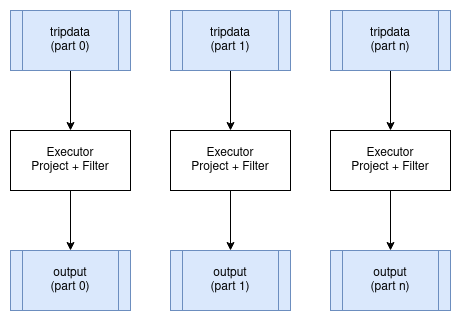
These operators are called "embarrassingly parallel" because parallelising them requires no special handling. The distributed plan looks just like the single-node plan, except different executors process different partitions. The partitioning scheme of the data does not change.
Distributed Aggregates
Aggregates require special handling in distributed execution. As discussed in the previous chapter, we split aggregation into two phases: a partial aggregate on each partition and a final aggregate that combines the partial results.
In distributed execution, the partial aggregates run on executors close to the data. The Exchange operator then moves partial results to where the final aggregation happens. For a query like:
SELECT passenger_count, MAX(fare_amount)
FROM tripdata
GROUP BY passenger_count
The distributed plan looks like:
HashAggregate: groupBy=[passenger_count], aggr=[MAX(fare_amount)]
  Exchange:
    HashAggregate: groupBy=[passenger_count], aggr=[MAX(fare_amount)]
      Scan: tripdata.parquet
Each executor runs the inner HashAggregate on its assigned partitions of tripdata. This produces partial results with far fewer rows than the input (one row per distinct passenger_count value per partition). The Exchange operator collects these partial results, and the outer HashAggregate combines them into the final answer.
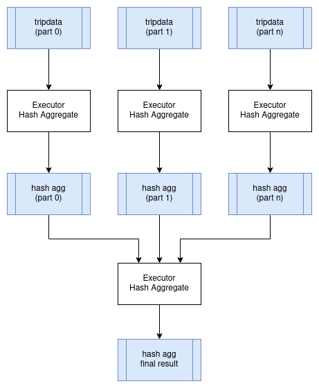
The exchange is the expensive part. Even though partial aggregation dramatically reduces data volume, we still need to transfer data over the network. For this query, we might reduce billions of input rows to thousands of partial aggregate rows, but those rows still need to reach whichever executor performs the final aggregation.
For aggregates grouped by high-cardinality columns (columns with many distinct values), the partial results may not be much smaller than the input. In extreme cases, the distributed overhead outweighs the benefit of distributing the initial scan.
Distributed Joins
Joins are often the most expensive operation in distributed query execution because they typically require shuffling large amounts of data across the network.
The challenge is that rows from both tables can only be joined if they are on the same executor. If we are joining customer to orders on customer.id = order.customer_id, then all orders for customer 12345 must be processed by the same executor that has customer 12345's details.
Shuffle Join
When both tables are large, we use a shuffle join (also called a partitioned hash join). Both tables are repartitioned by the join key, ensuring that matching rows end up on the same executor.
The process has two stages:
-
Shuffle stage: Read both tables and redistribute rows based on a hash of the join key. All rows with the same join key value go to the same partition, and thus the same executor. This requires transferring potentially large amounts of data across the network.
-
Join stage: Each executor performs a local hash join on its partitions. Since all matching rows are now local, no further network communication is needed.
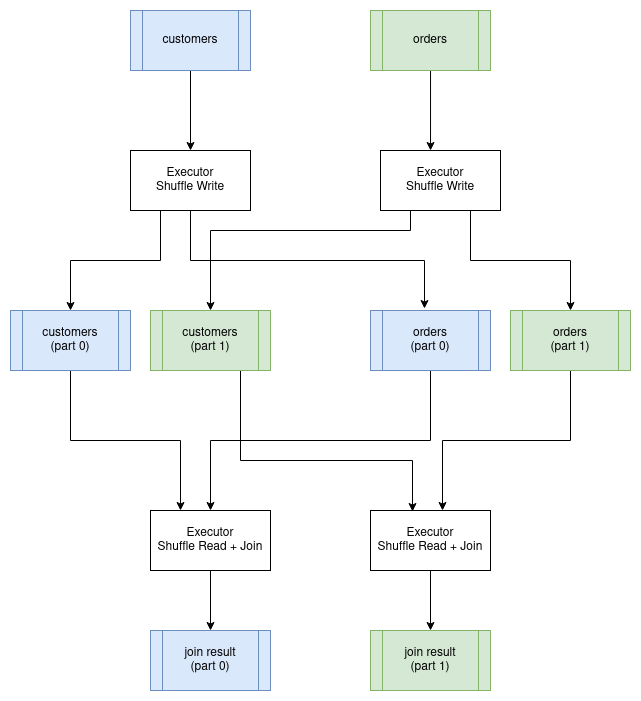
The shuffle is expensive. Every row from both tables must be sent over the network to its destination executor. For a join between two billion-row tables, this could mean transferring terabytes of data, even if the final result is small.
Broadcast Join
When one side of a join is small enough to fit in memory on each executor, we can avoid the shuffle entirely. The coordinator sends a copy of the small table to every executor. Each executor then joins its partitions of the large table against the local copy of the small table.
This trades network bandwidth (sending the small table everywhere) for avoiding the much larger cost of shuffling the big table. It only works when the small table is genuinely small, typically under a few gigabytes.
The query planner decides between shuffle and broadcast joins based on table size estimates. If statistics are available, it can make this decision automatically. Otherwise, users may need to provide hints.
Co-located Joins
If both tables are already partitioned by the join key (perhaps because they were written that way, or because a previous operation partitioned them), we can skip the shuffle entirely. Each executor joins its local partitions from both tables.
This is the fastest distributed join because no data moves. It requires careful data layout and is common in data warehouses where tables are deliberately partitioned by frequently-joined keys.
Query Stages
A distributed query cannot be executed as a single unit. The coordinator must break it into stages that can be executed independently, schedule those stages in the right order, and coordinate data flow between them.
A query stage is a portion of the query plan that can run to completion without waiting for other stages. Stages are separated by exchange operators, which represent points where data must be shuffled between executors. Within a stage, operators can be pipelined: data flows from one operator to the next without materialisation.
Consider the aggregate query from earlier:
HashAggregate: groupBy=[passenger_count], aggr=[MAX(fare_amount)]
  Exchange:
    HashAggregate: groupBy=[passenger_count], aggr=[MAX(fare_amount)]
      Scan: tripdata.parquet
This plan has two stages:
Stage 1: Scan the data and compute partial aggregates. This runs in parallel across all executors that have data partitions. Each executor reads its partitions, aggregates locally, and writes results to shuffle files.
Stage 2: Read the shuffle outputs from Stage 1 and compute the final aggregate. This might run on a single executor (for queries that need a single result) or on multiple executors (if the result is partitioned).
Stage 2 cannot start until Stage 1 completes because it reads Stage 1's output. The coordinator tracks stage dependencies and schedules stages as their inputs become available.
Producing a Distributed Query Plan
Converting a logical plan into a distributed execution plan involves identifying where exchanges must occur and grouping operators into stages. The boundaries between stages occur where data must be repartitioned.
Consider this query joining customers with their orders:
SELECT customer.id, SUM(order.amount) AS total_amount
FROM customer JOIN order ON customer.id = order.customer_id
GROUP BY customer.id
The single-node physical plan looks like:
Projection: #customer.id, #total_amount
  HashAggregate: groupBy=[customer.id], aggr=[SUM(amount) AS total_amount]
    Join: condition=[customer.id = order.customer_id]
      Scan: customer
      Scan: order
To distribute this, we need to identify where exchanges occur. Assuming the tables are not already partitioned by customer id, the join requires shuffling both tables. The aggregate can run partially on each executor, but needs a final aggregation.
Stage 1 and 2 (run in parallel): Read and shuffle the input tables.
Stage #1: repartition=[customer.id]
  Scan: customer

Stage #2: repartition=[order.customer_id]
  Scan: order
Stage 3: Join the shuffled data and compute partial aggregates. Since the data is now partitioned by customer id, matching rows from both tables are on the same executor.
Stage #3: repartition=[]
  HashAggregate: groupBy=[customer.id], aggr=[SUM(amount) AS total_amount]
    Join: condition=[customer.id = order.customer_id]
      Stage #1 output
      Stage #2 output
Stage 4: Combine partial aggregates and project the final result.
Stage #4:
  Projection: #customer.id, #total_amount
    HashAggregate: groupBy=[customer.id], aggr=[SUM(total_amount)]
      Stage #3 output
The execution order is: Stages 1 and 2 run in parallel, then Stage 3, then Stage 4. Each stage boundary is an exchange where data is either shuffled (for the join) or gathered (for the final aggregation).
Serializing a Query Plan
The query scheduler needs to send fragments of the overall query plan to executors for execution.
There are a number of options for serializing a query plan so that it can be passed between processes. Many query engines choose the strategy of using the programming language's native serialization support, which is a suitable choice if there is no requirement to exchange query plans between different programming languages and this is usually the simplest mechanism to implement.
However, there are advantages in using a serialization format that is programming language-agnostic. KQuery uses Google's Protocol Buffers format to define query plans. The project is typically abbreviated as "protobuf".
Here is a subset of KQuery's protocol buffer definition for physical plans, which is what the scheduler sends to executors.
Full source code can be found at protobuf/src/main/proto/kquery.proto in the KQuery GitHub repository.
message PhysicalPlanNode {
  oneof plan_type {
    ScanExecNode scan = 1;
    ProjectionExecNode projection = 2;
    SelectionExecNode selection = 3;
    HashAggregateExecNode hash_aggregate = 4;
    ShuffleWriterExecNode shuffle_writer = 10;
    ShuffleReaderExecNode shuffle_reader = 11;
  }
}

message ScanExecNode {
  string path = 1;
  Schema schema = 2;
  repeated string projection = 3;
  string file_format = 4;
}

message HashAggregateExecNode {
  PhysicalPlanNode input = 1;
  repeated PhysicalExprNode group_expr = 2;
  repeated PhysicalAggregateExprNode aggregate_expr = 3;
  Schema schema = 4;
  AggregateMode mode = 5;
}

enum AggregateMode {
  COMPLETE = 0;  // Single-node aggregation
  PARTIAL = 1;   // First stage: outputs intermediate state
  FINAL = 2;     // Second stage: merges intermediate states
}

message ShuffleWriterExecNode {
  PhysicalPlanNode input = 1;
  repeated PhysicalExprNode partition_expr = 2;
  string job_uuid = 3;
  int32 stage_id = 4;
  int32 partition_count = 5;
}

message ShuffleReaderExecNode {
  Schema schema = 1;
  repeated ShuffleLocation shuffle_locations = 2;
}
The AggregateMode enum is particularly important for distributed aggregation. In distributed mode, aggregates run in two stages: the first stage computes partial results (PARTIAL mode) on each executor, and the second stage merges those partial results (FINAL mode) to produce the final answer. This is how the "map-reduce" pattern from the previous chapter is implemented.
The protobuf project provides tools for generating language-specific source code for serializing and de-serializing data. KQuery includes PhysicalPlanSerializer and PhysicalPlanDeserializer classes that convert between the in-memory physical plan representation and the protobuf format.
Serializing Data
Data must also be serialized as it is streamed between clients and executors and between executors.
Apache Arrow provides an IPC (Inter-process Communication) format for exchanging data between processes. Because of the standardized memory layout provided by Arrow, the raw bytes can be transferred directly between memory and an input/output device (disk, network, etc) without the overhead typically associated with serialization. This is effectively a zero copy operation because the data does not have to be transformed from its in-memory format to a separate serialization format.
However, the metadata about the data, such as the schema (column names and data types) does need to be encoded using Google Flatbuffers. This metadata is small and is typically serialized once per result set or per batch so the overhead is small.
Another advantage of using Arrow is that it provides very efficient exchange of data between different programming languages.
Apache Arrow IPC defines the data encoding format but not the mechanism for exchanging it. Arrow IPC could be used to transfer data from a JVM language to C or Rust via JNI for example.
Choosing a Protocol
Now that we have chosen serialization formats for query plans and data, the next question is how do we exchange this data between distributed processes.
Apache Arrow provides a Flight protocol which is intended for this exact purpose. Flight is a new general-purpose client-server framework to simplify high performance transport of large datasets over network interfaces.
The Arrow Flight libraries provide a development framework for implementing a service that can send and receive data streams. A Flight server supports several basic kinds of requests:
- Handshake: a simple request to determine whether the client is authorized and, in some cases, to establish an implementation-defined session token to use for future requests
- ListFlights: return a list of available data streams
- GetSchema: return the schema for a data stream
- GetFlightInfo: return an “access plan” for a dataset of interest, possibly requiring consuming multiple data streams. This request can accept custom serialized commands containing, for example, your specific application parameters.
- DoGet: send a data stream to a client
- DoPut: receive a data stream from a client
- DoAction: perform an implementation-specific action and return any results, i.e. a generalized function call
- ListActions: return a list of available action types
The GetFlightInfo method could be used to compile a query plan and return the necessary information for receiving the results, for example, followed by calls to DoGet on each executor to start receiving the results from the query.
Streaming vs Blocking Operators
Operators differ in whether they can stream results incrementally or must wait for all input before producing output.
Streaming operators produce output as soon as they receive input. Filter and projection are streaming: each input batch produces an output batch immediately. A pipeline of streaming operators can begin returning results while still reading input, reducing latency and memory usage.
Blocking operators must receive all input before producing any output. Sort is the clearest example: you cannot know which row comes first until you have seen all rows. Global aggregates (without GROUP BY) are similar: you cannot return the final SUM until all rows are processed.
Partially blocking operators fall in between. Hash join builds a hash table from one input (blocking on that side) but then streams through the other input. Hash aggregate accumulates results but can output partial aggregates incrementally when using two-phase aggregation.
In distributed execution, blocking operators create natural stage boundaries. All upstream work must complete before the blocking operator can produce its first output. This affects both latency (how long until results start appearing) and resource usage (intermediate data must be materialised).
Increasing the number of partitions helps reduce blocking time. Instead of one executor sorting a billion rows, we have a thousand executors each sorting a million rows. The merge step at the end is still necessary, but it operates on pre-sorted streams and can begin producing output immediately.
Data Locality
A key optimisation in distributed execution is moving computation to data rather than data to computation. Reading a terabyte over the network takes far longer than running a query locally on a terabyte of data.
When data lives in a distributed file system like HDFS, the coordinator knows which machines have local copies of each data block. It can assign tasks to executors that have the data locally, avoiding network transfer for the initial scan. This is called data locality or data affinity.
With cloud object stores like S3, data locality is less relevant because data must be fetched over the network regardless. However, executors in the same region as the storage will have lower latency and higher bandwidth than executors in different regions.
The shuffle operation between stages necessarily moves data across the network, so data locality only helps with the initial scan. For queries that are dominated by shuffles (complex joins, high-cardinality aggregates), locality provides less benefit.
Fault Tolerance
Long-running distributed queries face a significant risk: with hundreds of machines running for hours, the probability that at least one fails becomes high. Without fault tolerance, any failure means restarting the entire query from scratch.
There are several approaches to fault tolerance:
Checkpointing: Periodically save intermediate state to durable storage. If a failure occurs, restart from the most recent checkpoint rather than from the beginning. The trade-off is the overhead of writing checkpoints.
Lineage-based recovery: Instead of saving intermediate data, save the computation graph (lineage) that produced it. If data is lost, recompute it from its inputs. This is the approach used by Apache Spark. It works well when the lineage is not too long and recomputation is cheap.
Replication: Run multiple copies of each task on different machines. If one fails, use the results from another. This trades resource efficiency for reliability and is typically used for critical stages.
Task retry: If a task fails, simply re-run it (possibly on a different executor). This works for transient failures but requires the input data to still be available.
Most production systems combine these approaches. Early stages use lineage-based recovery (input data is durable on disk, so lost results can be recomputed). Expensive shuffle data may be replicated or checkpointed. Failed tasks are retried a few times before escalating to stage-level recovery.
Custom Code
It is often necessary to run user-defined functions as part of a distributed query. Serializing and shipping code to executors raises practical challenges.
For single-language systems, the language's built-in serialization often works. Java can serialize lambda functions, Python can pickle functions (with caveats). The coordinator sends the serialized code along with the query plan.
For production systems, code is typically pre-deployed to executors. JVM systems might use Maven coordinates to download JARs. Container-based systems package dependencies into Docker images. The query plan then references the code by name rather than including it inline.
The user code must implement a known interface so the executor can invoke it. Type mismatches between the expected and actual interfaces cause runtime failures that can be hard to debug in a distributed setting.
Distributed Query Optimizations
The same query can be distributed in many ways. Choosing the best distribution requires estimating costs and making trade-offs.
Cost Factors
Distributed execution involves multiple scarce resources:
Network bandwidth: Shuffles transfer data between machines. Network is often the bottleneck, especially for join-heavy queries. Minimising shuffle size is usually the highest priority.
Memory: Each executor has limited memory. Hash tables for joins and aggregates must fit, or spill to disk at a severe performance cost. More executors means more aggregate memory, but also more coordination overhead.
CPU: Computation itself is parallelisable, but the benefit diminishes if the query is bottlenecked on I/O or network.
Disk I/O: Reading source data, writing shuffle files, and spilling all compete for disk bandwidth. SSDs help but have limits.
Monetary cost: In cloud environments, more executors means higher cost. A query that runs in 10 minutes on 100 executors might run in 15 minutes on 50 executors at half the price.
Optimisation Strategies
Shuffle minimisation: Choose join strategies that minimise data movement. Use broadcast joins when one side is small. Leverage co-located data when available. Filter early to reduce the data that reaches shuffles.
Predicate pushdown: Push filters as close to the data source as possible. If the storage system supports predicate pushdown (like Parquet with column statistics), even less data is read from disk.
Partition pruning: Skip partitions that cannot contain matching rows. Time-partitioned data benefits enormously when queries filter on time.
Statistics-based planning: With accurate statistics (row counts, column cardinalities, value distributions), the planner can estimate costs and choose better strategies. Without statistics, it must guess or use conservative defaults.
Adaptive Execution
An alternative to upfront cost estimation is adaptive execution: start running the query and adjust the plan based on observed data characteristics.
Apache Spark's Adaptive Query Execution dynamically:
- Coalesces small shuffle partitions to reduce overhead
- Switches join strategies based on actual data sizes
- Optimises skewed joins by splitting hot partitions
Adaptive execution is particularly valuable when statistics are unavailable or stale, which is common in data lake environments where new data arrives continuously.
The COST of Distribution
It bears repeating: distributed execution has overhead. The paper "Scalability! But at what COST?" (Configuration that Outperforms a Single Thread) demonstrates that many distributed systems are slower than a single well-optimised machine for medium-sized datasets.
Before scaling out to a cluster, ensure you have actually hit the limits of a single machine. Modern servers with hundreds of gigabytes of RAM and fast NVMe storage can process surprisingly large datasets. The complexity and operational overhead of distributed systems is only justified when the data truly exceeds single-machine capacity.
KQuery Distributed Implementation
KQuery includes a distributed execution module that demonstrates the concepts discussed in this chapter. While simplified compared to production systems, it illustrates the key components: a scheduler that plans queries into stages, executors that run tasks, and shuffle operations that exchange data between stages.
Distributed Planner
The DistributedPlanner converts a physical plan into query stages separated by shuffle boundaries. For aggregate queries, it produces two stages:
Source code can be found at distributed/src/main/kotlin/io/andygrove/kquery/distributed/DistributedPlanner.kt
fun plan(plan: PhysicalPlan, jobUuid: String): List<QueryStage> {
  return when (plan) {
    is HashAggregateExec -> planAggregate(plan, jobUuid)
    else -> {
      // For non-aggregate plans, wrap in a single stage
      listOf(QueryStage(stageId = 0, plan = plan, isFinalStage = true))
    }
  }
}

private fun planAggregate(
    aggregate: HashAggregateExec,
    jobUuid: String
): List<QueryStage> {
  // Stage 0: Partial aggregation with shuffle write
  val partialAggregate = HashAggregateExec(
      input = aggregate.input,
      groupExpr = aggregate.groupExpr,
      aggregateExpr = aggregate.aggregateExpr,
      schema = aggregate.schema,
      mode = AggregateMode.PARTIAL)

  val shuffleWriter = ShuffleWriterExec(
      input = partialAggregate,
      partitionExpr = aggregate.groupExpr,
      jobUuid = jobUuid,
      stageId = 0,
      partitionCount = config.getPartitionCount())

  // Stage 1: Shuffle read with final aggregation
  val shuffleReader = ShuffleReaderExec(
      shuffleSchema = aggregate.schema,
      shuffleLocations = listOf())

  val finalAggregate = HashAggregateExec(
      input = shuffleReader,
      groupExpr = aggregate.groupExpr,
      aggregateExpr = aggregate.aggregateExpr,
      schema = aggregate.schema,
      mode = AggregateMode.FINAL)

  return listOf(
      QueryStage(stageId = 0, plan = shuffleWriter, ...),
      QueryStage(stageId = 1, plan = finalAggregate, ...)
  )
}
Scheduler
The scheduler orchestrates execution by assigning tasks to executors and coordinating stage dependencies:
Source code can be found at distributed/src/main/kotlin/io/andygrove/kquery/distributed/Scheduler.kt
fun execute(plan: PhysicalPlan): Sequence<RecordBatch> {
  val jobUuid = UUID.randomUUID().toString()
  val stages = planner.plan(plan, jobUuid)

  var shuffleLocations = listOf<ShuffleLocation>()

  for (stage in stages) {
    val stageWithLocations =
        planner.updateShuffleLocations(stage, shuffleLocations)

    if (stage.isFinalStage) {
      return executeFinalStage(stageWithLocations)
    } else {
      shuffleLocations = executeStage(stageWithLocations)
    }
  }
  return emptySequence()
}
Example Usage
The DistributedContext provides a high-level API similar to ExecutionContext:
Source code can be found at examples/src/main/kotlin/DistributedExample.kt
// Configure a cluster with 3 executors
val config = DistributedConfig(
    executors = listOf(
        ExecutorConfig("exec-1", "localhost", 50051),
        ExecutorConfig("exec-2", "localhost", 50052),
        ExecutorConfig("exec-3", "localhost", 50053)))

val ctx = DistributedContext(config, executorClient)
ctx.registerCsv("employee", employeeCsv)

val results = ctx.sql(
    "SELECT state, SUM(salary) FROM employee GROUP BY state")
When this query executes:
- The planner creates two stages: partial aggregation with shuffle write, and final aggregation with shuffle read.
- Stage 0 tasks are distributed across the three executors. Each executor reads its partition of the data, computes partial aggregates, and writes shuffle files.
- Stage 1 reads the shuffle outputs and merges them into the final result.
The shuffle data is exchanged using Apache Arrow's IPC format, which allows efficient serialization of columnar data. In a real deployment, executors would communicate via Arrow Flight; the example includes a local executor client for testing.
This book is also available for purchase in ePub, MOBI, and PDF format from https://leanpub.com/how-query-engines-work
Copyright © 2020-2026 Andy Grove. All rights reserved.