Acknowledgments

This book would not have been possible without the support of my family, who are incredibly patient with me when I get absorbed with yet another side project.

Special thanks go to Matthew Powers, a.k.a. Mr. Powers, for inspiring me to write this book in the first place. Matthew is the author of the book “Writing Beautiful Apache Spark Code” which is also available on Leanpub.

I also need to thank the countless people who have interacted with me over the past six years as I worked on the DataFusion project, especially the Apache Arrow and Apache DataFusion PMC members, committers, and contributors. This book would not have been possible without you.

This book is also available for purchase in ePub, MOBI, and PDF format from https://leanpub.com/how-query-engines-work

Preface

The first edition of this book was written in a one week break between jobs and improved during COVID lockdown in 2020. I honestly wasn’t sure how many people wanted to read a book about building a query engine from scratch. It turns out that there are quite a few.

This second edition is a significant revision with clearer explanations, better code organization, and expanded coverage of topics like joins, subqueries, and distributed query execution.

This book is not academic in nature. It aims to be a practical, straightforward guide. The feedback from readers has been encouraging, so thank you to everyone who provided suggestions and corrections. I hope this edition serves as an even better foundation for understanding query engines.

Feedback

I welcome feedback on this book. You can contact me on LinkedIn or through the Leanpub forum.

This book is also available for purchase in ePub, MOBI, and PDF format from https://leanpub.com/how-query-engines-work

Introduction

Query engines are the invisible workhorses powering modern data infrastructure. Every time you run a SQL query against a database, execute a Spark job, or query a data lake, a query engine is transforming your high-level request into an efficient execution plan. Understanding how query engines work gives you insight into one of the most important abstractions in computing.

This book takes a hands-on approach to demystifying query engines. Rather than surveying existing systems, we will build a fully functional query engine from scratch, covering each component in enough depth that you could implement your own.

Who This Book Is For

This book is for software engineers who want to understand the internals of query engines. You might be:

A data engineer who wants to understand why queries perform the way they do
A database developer looking to learn foundational concepts
A software engineer curious about compiler-like systems
Someone building tooling that needs to parse or analyze SQL

Basic programming knowledge is assumed. The examples use Kotlin, chosen for its conciseness, but the concepts apply to any language.

What You Will Learn

By the end of this book, you will understand how to:

Design a columnar type system using Apache Arrow
Build data source connectors for CSV and Parquet files
Represent queries as logical and physical plans
Create a DataFrame API for building queries programmatically
Translate logical plans into executable physical plans
Implement query optimizations like projection and predicate push-down
Parse SQL and convert it to query plans
Execute queries in parallel across multiple CPU cores
Design distributed query execution across a cluster

How This Book Is Organized

The book follows the natural architecture of a query engine, building each layer on top of the previous.

Chapters 1 through 4 cover the foundations. We start with what a query engine is, then establish our foundation with Apache Arrow for the memory model, a type system for representing data, and data source abstractions for reading files.

Chapters 5 through 7 cover query representation. We define logical plans and expressions to represent queries abstractly, build a DataFrame API for constructing plans programmatically, and add SQL support so queries can be written in the familiar query language.

Chapters 8 through 10 cover execution. We translate logical plans into physical plans containing executable code, then cover joins and subqueries, two of the most complex operations in query processing.

Chapters 11 through 13 cover planning and optimization. We implement a query planner to automate the translation from logical to physical plans, build optimizer rules to transform plans into more efficient forms, and execute queries to compare performance.

Chapters 14 and 15 cover scaling. We extend the engine to execute queries in parallel across CPU cores, then across distributed clusters.

Chapters 16 and 17 cover quality. We cover testing strategies including fuzzing, and benchmarking approaches for measuring performance.

This book is also available for purchase in ePub, MOBI, and PDF format from https://leanpub.com/how-query-engines-work

The KQuery Project

This book is accompanied by a fully functional query engine called KQuery (for Kotlin Query). The source code is available on GitHub:

https://github.com/andygrove/how-query-engines-work

Each chapter references specific modules in this repository. Reading the book alongside the code will deepen your understanding. The book explains the design decisions, while the code shows the complete implementation.

Why Kotlin?

The examples use Kotlin because it is concise and readable. If you know Java, Python, or any C-family language, you will follow along easily. Kotlin runs on the JVM and interoperates seamlessly with Java libraries like Apache Arrow.

Query engine concepts are language-agnostic. The Apache Arrow DataFusion project implements similar ideas in Rust, and you could apply these patterns in any language.

Repository Structure

The repository is organized into Gradle modules, each corresponding to a layer of the query engine:

Module	Description
`datatypes`	Type system built on Apache Arrow
`datasource`	Data source abstractions and CSV/Parquet readers
`logical-plan`	Logical plans and expressions
`physical-plan`	Physical plans and expression evaluation
`query-planner`	Translation from logical to physical plans
`optimizer`	Query optimization rules
`sql`	SQL tokenizer, parser, and planner
`execution`	Query execution engine
`examples`	Example queries and benchmarks

Building the Project

Prerequisites:

JDK 11 or later
Gradle (or use the included Gradle wrapper)

To build and run tests:

cd jvm
./gradlew build

To run a specific test:

./gradlew :sql:test --tests "SqlParserTest"

Running Examples

The examples module contains sample queries you can run:

./gradlew :examples:run

See the README in the repository for the latest instructions and any additional setup required.

This book is also available for purchase in ePub, MOBI, and PDF format from https://leanpub.com/how-query-engines-work

What Is a Query Engine?

If you have written code to search through a list or filter items in an array, you have already implemented a tiny query engine. A query engine is simply software that retrieves and processes data based on some criteria. The difference between your for loop and a production query engine is scale, generality, and optimization, but the core idea is the same.

Consider this Python code that finds all students with a GPA above 3.5:

high_achievers = []
for student in students:
    if student.gpa > 3.5:
        high_achievers.append(student)

This is querying data. Now imagine you need to do this across millions of records stored in files, join data from multiple sources, group results, and compute aggregates, all while keeping response times reasonable. That is what query engines do.

From Code to Queries

The code above works, but it has limitations. What if you want to change the filter condition? You would need to modify and recompile the code. What if someone without programming experience needs to analyze the data?

Query languages like SQL solve this by providing a declarative way to express what data you want, without specifying how to get it:

SELECT name, gpa
FROM students
WHERE gpa > 3.5;

This query expresses the same logic as our Python loop, but the query engine decides how to execute it efficiently. This separation of “what” from “how” is powerful. The same query can run against a small file or a distributed cluster of servers.

Anatomy of a Query Engine

A query engine transforms a query (like the SQL above) into actual results through several stages:

Parsing: Convert the query text into a structured representation (like an abstract syntax tree)
Planning: Determine which operations are needed (scan, filter, join, aggregate)
Optimization: Reorder and transform operations for efficiency
Execution: Actually process the data and produce results

This pipeline might remind you of a compiler, and that is no coincidence. Query engines are essentially specialized compilers that translate declarative queries into efficient execution plans.

A Concrete Example

Let us look at a slightly more complex query:

SELECT department, AVG(salary)
FROM employees
WHERE hire_date > '2020-01-01'
GROUP BY department
ORDER BY AVG(salary) DESC;

This query:

Scans the employees table
Filters to only recent hires
Groups employees by department
Computes the average salary per department
Sorts results by that average

A query engine must determine the most efficient way to execute these operations. Should it filter before or after grouping? How should it store intermediate results? These decisions significantly impact performance, especially with large datasets.

SQL: The Universal Query Language

SQL (Structured Query Language) has been the dominant query language since the 1970s. You will encounter it in:

Relational databases (PostgreSQL, MySQL, SQLite)
Data warehouses (Snowflake, BigQuery, Redshift)
Big data systems (Apache Spark, Presto, Hive)
Even embedded analytics (DuckDB)

Here are two more examples showing SQL’s expressiveness:

Finding the top 5 most visited pages yesterday:

SELECT page_url, COUNT(*) AS visits
FROM page_views
WHERE view_date = CURRENT_DATE - 1
GROUP BY page_url
ORDER BY visits DESC
LIMIT 5;

Calculating month-over-month growth:

SELECT month, revenue,
       revenue - LAG(revenue) OVER (ORDER BY month) AS growth
FROM monthly_sales
WHERE year = 2024;

Beyond SQL: DataFrame APIs

Whilst SQL is ubiquitous, many query engines also provide programmatic APIs. These are especially popular in data science where queries are often built dynamically or mixed with custom code.

Here is the same query expressed using Apache Spark’s DataFrame API in Scala:

val spark = SparkSession.builder
  .appName("Example")
  .master("local[*]")
  .getOrCreate()

val result = spark.read.parquet("/data/employees")
  .filter($"hire_date" > "2020-01-01")
  .groupBy("department")
  .agg(avg("salary").as("avg_salary"))
  .orderBy(desc("avg_salary"))

result.show()

The DataFrame API provides the same logical operations as SQL but expressed as method calls. Under the hood, both approaches generate the same query plan.

Why Build a Query Engine?

Understanding query engines helps you:

Write better queries, because knowing how queries execute helps you write efficient ones
Debug performance issues, because understanding the optimizer helps diagnose slow queries
Appreciate database internals, because query engines are at the heart of every database
Build data tools, because many applications need query-like functionality

Query engines also touch many areas of computer science: parsing and compilers, data structures, algorithms, distributed systems, and optimization. Building one is excellent practice.

What This Book Covers

This book walks through building a complete query engine from scratch. We will implement:

A type system for representing data
Data source connectors for reading files
Logical and physical query plans
A SQL parser and planner
Query optimization rules
Parallel and distributed execution

The query engine (called KQuery) is intentionally simple, optimized for learning rather than production use. But the concepts apply directly to real systems like Apache Spark, Presto, and DataFusion.

This book is also available for purchase in ePub, MOBI, and PDF format from https://leanpub.com/how-query-engines-work

Apache Arrow

Before we start building our query engine, we need to choose how to represent data in memory. This choice affects everything: how we read files, how we pass data between operators, and how fast our computations run. We will use Apache Arrow, which has become the standard for in-memory columnar data.

Why Columnar?

Traditional databases and programming languages typically store data row by row. If you have a table of employees, each employee record sits together in memory:

Row 0: [1, "Alice", "Engineering", 95000]
Row 1: [2, "Bob", "Sales", 87000]
Row 2: [3, "Carol", "Engineering", 102000]

This layout is intuitive and works well when you need to access entire records. But query engines often process just a few columns at a time. Consider:

SELECT AVG(salary) FROM employees WHERE department = 'Engineering'

This query only needs the department and salary columns. With row-based storage, we would load entire rows into memory just to access two fields.

Columnar storage flips this around. Each column is stored contiguously:

ids:         [1, 2, 3]
names:       ["Alice", "Bob", "Carol"]
departments: ["Engineering", "Sales", "Engineering"]
salaries:    [95000, 87000, 102000]

Now reading salary means reading one contiguous block of memory, with no jumping around to skip unwanted fields. This matters enormously for performance:

Modern CPUs load memory in cache lines (typically 64 bytes). Columnar data packs more useful values per cache line.
Similar values grouped together compress much better. A column of departments might compress to just a few distinct values.
CPUs can apply the same operation to multiple values simultaneously (Single Instruction, Multiple Data). Columnar layout enables this.

What Is Apache Arrow?

Apache Arrow is a specification for how to represent columnar data in memory, plus libraries implementing that specification in many languages. Think of it as a universal format that different systems can share.

The key insight behind Arrow is that data analytics involves many tools: Python for exploration, Spark for distributed processing, databases for storage, visualization tools for presentation. Traditionally, each tool has its own internal format, so moving data between tools means serializing and deserializing, converting formats repeatedly.

Arrow eliminates this overhead. If your Python code and your Java code both use Arrow format, they can share memory directly. A pointer to Arrow data is meaningful to any Arrow-aware system.

Arrow Memory Layout

An Arrow column (called a “vector” or “array”) consists of:

A data buffer containing the actual values, packed contiguously
A validity buffer, which is a bitmap indicating which values are null
An optional offset buffer for variable-length types like strings

For a column of 32-bit integers [1, null, 3, 4]:

Validity bitmap: [1, 0, 1, 1]  (bit per value: 1=valid, 0=null)
Data buffer:     [1, ?, 3, 4]  (? = undefined, since null)

For strings, we need offsets because strings vary in length:

Values: ["hello", "world", "!"]

Offsets: [0, 5, 10, 11]  (start position of each string, plus end)
Data:    "helloworld!"   (all strings concatenated)

To get string at index 1: read from offset[1]=5 to offset[2]=10, giving “world”.

This layout is simple but powerful. Fixed-width types like integers require just one memory access per value. The validity bitmap uses just one bit per value, so checking for nulls is cheap.

Record Batches

A single column is not very useful on its own. We need multiple columns together. Query engines typically group columns into record batches: a collection of equal-length columns with a schema describing their names and types. KQuery defines its own RecordBatch class for this purpose.

RecordBatch:
  Schema: {id: Int32, name: Utf8, salary: Float64}
  Columns:
    id:     [1, 2, 3]
    name:   ["Alice", "Bob", "Carol"]
    salary: [95000.0, 87000.0, 102000.0]
  Length: 3

Query engines process data in batches rather than row by row or all at once. Batch processing hits the sweet spot:

Small enough to fit in CPU cache
Large enough to amortize per-batch overhead
Enables streaming (process data as it arrives)

Typical batch sizes range from 1,000 to 100,000 rows depending on the workload.

Schemas and Types

Arrow defines a rich type system covering:

Integers: Int8, Int16, Int32, Int64 (signed and unsigned)
Floating point: Float32 (single), Float64 (double)
Binary: Variable-length byte arrays
Strings: UTF-8 encoded text
Temporal: Date, Time, Timestamp, Duration, Interval
Nested: List, Struct, Map, Union

A schema names and types the columns:

Schema:
  - id: Int32, not nullable
  - name: Utf8, nullable
  - hire_date: Date32, nullable
  - salary: Float64, not nullable

Having explicit nullability in the schema lets the query engine optimize. If a column cannot be null, we can skip null checks entirely.

Language Implementations

Arrow has official implementations in C++, Java, Python, Rust, Go, JavaScript, C#, Ruby, and more. For this book, we will use the Java implementation.

The Java API provides:

FieldVector: Base class for column vectors (IntVector, VarCharVector, etc.)
VectorSchemaRoot: Container for a record batch
ArrowType: Represents data types
Schema/Field: Describes the structure of data

Here is a simple example creating an Arrow vector in Java:

try (IntVector vector = new IntVector("id", allocator)) {
    vector.allocateNew(3);
    vector.set(0, 1);
    vector.set(1, 2);
    vector.set(2, 3);
    vector.setValueCount(3);
    // vector now contains [1, 2, 3]
}

Why Arrow for Our Query Engine?

We will use Arrow as the foundation of our query engine for several reasons:

It is a standard format, so we can easily read/write Parquet files and integrate with other tools
The Java library is mature and well-tested
The columnar layout enables efficient query processing
Understanding Arrow helps you understand other data systems

The next chapter builds our type system on top of Arrow, adding the abstractions our query engine needs.

Type System

The source code discussed in this chapter can be found in the datatypes module of the KQuery project.

Every query engine needs a type system—a way to represent and reason about data types. When you write SELECT price * quantity, the engine must know that price and quantity are numbers that can be multiplied, and what type the result will be. This chapter builds KQuery’s type system on top of Apache Arrow.

Why Types Matter

Consider this query:

SELECT name, salary * 1.1 AS new_salary
FROM employees
WHERE department = 'Engineering'

Before executing, the query engine must answer:

Is salary a numeric type that supports multiplication?
What’s the result type of salary * 1.1? (If salary is an integer, should the result be integer or floating point?)
Is department a string type that supports equality comparison?
What columns and types does the result have?

These questions arise during query planning, before we touch any data. A well-designed type system catches errors early (“you can’t multiply a string by a number”) and enables optimizations (“this column is never null, so skip null checks”).

Building on Arrow

Rather than invent our own type system, we’ll use Apache Arrow’s types directly. This gives us:

A rich set of standard types (integers, floats, strings, dates, etc.)
Efficient in-memory representation (as covered in the previous chapter)
Compatibility with Arrow-based tools and file formats

Arrow’s type system includes:

Category	Types
Boolean	Bool
Integers	Int8, Int16, Int32, Int64 (signed and unsigned)
Floating point	Float32, Float64
Text	Utf8 (variable-length strings)
Binary	Binary (variable-length bytes)
Temporal	Date32, Date64, Timestamp, Time32, Time64, Duration
Nested	List, Struct, Map

For KQuery, we’ll focus on the common types: booleans, integers, floating point numbers, and strings. We define convenient constants for these:

object ArrowTypes {
    val BooleanType = ArrowType.Bool()
    val Int8Type = ArrowType.Int(8, true)
    val Int16Type = ArrowType.Int(16, true)
    val Int32Type = ArrowType.Int(32, true)
    val Int64Type = ArrowType.Int(64, true)
    val UInt8Type = ArrowType.Int(8, false)
    val UInt16Type = ArrowType.Int(16, false)
    val UInt32Type = ArrowType.Int(32, false)
    val UInt64Type = ArrowType.Int(64, false)
    val FloatType = ArrowType.FloatingPoint(FloatingPointPrecision.SINGLE)
    val DoubleType = ArrowType.FloatingPoint(FloatingPointPrecision.DOUBLE)
    val StringType = ArrowType.Utf8()
}

Schemas and Fields

A schema describes the structure of a dataset: what columns exist and what type each has. Schemas are essential metadata that flows through the entire query engine.

Arrow represents schemas as a list of fields, where each field has:

A name (string)
A data type (ArrowType)
A nullable flag (can this column contain nulls?)

For example, an employee table might have this schema:

Schema:
  - id: Int32, not nullable
  - name: Utf8, nullable
  - department: Utf8, nullable
  - salary: Float64, not nullable

Schemas serve multiple purposes:

Validation: Reject queries that reference non-existent columns or misuse types
Planning: Determine output types for expressions
Optimization: Skip null checks for non-nullable columns
Execution: Allocate correctly-typed storage for results

Column Vectors

Arrow stores column data in vectors (also called arrays). Each vector type has its own class: IntVector, Float8Vector, VarCharVector, etc. This is efficient but inconvenient—code that processes columns would need type-specific branches everywhere.

KQuery introduces a ColumnVector interface to abstract over the underlying Arrow vectors:

/** Abstraction over different implementations of a column vector. */
interface ColumnVector : AutoCloseable {
  fun getType(): ArrowType

  fun getValue(i: Int): Any?

  fun size(): Int
}

This interface lets us write generic code that works with any column type. The getValue method returns Any? (Kotlin’s equivalent of Java’s Object), which isn’t ideal for performance but keeps our code simple.

We can wrap an Arrow FieldVector in this interface:

/** Wrapper around Arrow FieldVector */
class ArrowFieldVector(val field: FieldVector) : ColumnVector {

  override fun getType(): ArrowType {
    return when (field) {
      is BitVector -> ArrowTypes.BooleanType
      is TinyIntVector -> ArrowTypes.Int8Type
      is SmallIntVector -> ArrowTypes.Int16Type
      ...
      else -> throw IllegalStateException("Unsupported vector type: ${field.javaClass.name}")
    }
  }

  override fun getValue(i: Int): Any? {

    if (field.isNull(i)) {
      return null
    }

    return when (field) {
      is BitVector -> if (field.get(i) == 1) true else false
      is TinyIntVector -> field.get(i)
      is SmallIntVector -> field.get(i)
      ...
      else -> throw IllegalStateException("Unsupported vector type: ${field.javaClass.name}")
    }
  }

  override fun size(): Int {
    return field.valueCount
  }

  override fun close() {
    field.close()
  }
}

Literal Values

Sometimes we need a “column” that contains the same value repeated. For example, when evaluating salary * 1.1, the literal 1.1 needs to act like a column of 1.1 values (one per row in the batch).

Rather than allocate memory for thousands of identical values, we create a virtual column:

class LiteralValueVector(
    private val arrowType: ArrowType,
    private val value: Any?,
    private val size: Int
) : ColumnVector {

    override fun getType(): ArrowType = arrowType

    override fun getValue(i: Int): Any? {
        if (i < 0 || i >= size) {
            throw IndexOutOfBoundsException()
        }
        return value
    }

    override fun size(): Int = size
}

This returns the same value for any valid index, using constant memory regardless of how many rows we’re processing.

Record Batches

A record batch groups multiple columns together with a schema. This is the fundamental unit of data that flows through our query engine.

class RecordBatch(
    val schema: Schema,
    val fields: List<ColumnVector>
) {
    fun rowCount(): Int = fields.first().size()

    fun columnCount(): Int = fields.size

    fun field(i: Int): ColumnVector = fields[i]
}

Record batches enable batch processing: rather than processing one row at a time (slow due to function call overhead) or loading entire datasets into memory (impractical for large data), we process chunks of typically 1,000 to 100,000 rows.

Type Coercion

Real query engines need type coercion: automatically converting types when necessary. For example:

5 + 3.14 should promote the integer 5 to a float
Comparing Int32 to Int64 should work without explicit casts
String-to-date conversion for predicates like date > '2024-01-01'

KQuery keeps things simple and requires explicit types in most cases. A production query engine would implement coercion rules, typically promoting to the “wider” type (Int32 → Int64 → Float64).

Putting It Together

Here’s how these pieces fit together. When processing a query:

Data sources provide schemas describing available columns
Query planning uses schemas to validate expressions and determine result types
Execution passes record batches between operators
Each operator produces output batches with a known schema

The type system is the foundation that makes this possible. Without it, we couldn’t validate queries, plan efficiently, or allocate storage correctly.

The next chapter builds on this foundation to create abstractions for reading data from files.

This book is also available for purchase in ePub, MOBI, and PDF format from https://leanpub.com/how-query-engines-work

Data Sources

The source code discussed in this chapter can be found in the datasource module of the KQuery project.

A query engine needs data to query. The data might come from CSV files, Parquet files, databases, or even data that already exists in memory. We want our query engine to work with any of these without caring about the details. This chapter introduces the data source abstraction that makes this possible.

Why Abstract Data Sources?

Consider a simple query:

SELECT name, salary FROM employees WHERE department = 'Engineering'

From the query engine’s perspective, it needs to:

Know what columns exist (to validate that name, salary, and department are real)
Know the types of those columns (to validate that comparing department to a string makes sense)
Read the actual data, preferably just the columns it needs

Whether employees is a CSV file, a Parquet file, or an in-memory table, these requirements are the same. By defining a common interface, we can write query planning and execution logic once and have it work with any data source.

The DataSource Interface

KQuery defines a simple interface that all data sources must implement:

interface DataSource {

  / Return the schema for the underlying data source */
  fun schema(): Schema

  / Scan the data source, selecting the specified columns */
  fun scan(projection: List<String>): Sequence<RecordBatch>
}

schema() returns the schema of the data, the column names and their types. The query planner uses this during planning to validate queries. If you reference a column that does not exist, the planner can report an error before execution begins.

scan(projection) reads the data and returns it as a sequence of record batches. The projection parameter lists which columns to read. This is important for efficiency: if a query only uses three columns from a table with fifty columns, we should only read those three. Some file formats like Parquet support this natively. For others like CSV, we might read everything but only build vectors for the requested columns.

The return type Sequence<RecordBatch> enables streaming. Rather than loading an entire file into memory, we can process it batch by batch. This matters when data is larger than available memory.

CSV Data Source

CSV is the simplest format to understand but has some awkward properties. The file is just text with values separated by commas (or tabs, or semicolons). There is no schema embedded in the file, only optional column names in the first row.

Here is what a CSV file might look like:

id,name,department,salary
1,Alice,Engineering,95000
2,Bob,Sales,87000
3,Carol,Engineering,102000

To read this, we need to handle several things:

Parse column names from the header row (if present)
Infer or accept a schema (what types are these columns?)
Parse text values into typed values
Handle missing or malformed values

KQuery’s CsvDataSource accepts an optional schema. If provided, it uses that schema. If not, it infers one by reading the header row and treating all columns as strings:

class CsvDataSource(
    val filename: String,
    val schema: Schema?,
    private val hasHeaders: Boolean,
    private val batchSize: Int
) : DataSource {

  private val finalSchema: Schema by lazy { schema ?: inferSchema() }

  override fun schema(): Schema {
    return finalSchema
  }
  // ...
}

The scan method streams through the file, parsing rows into batches. For each batch, it creates Arrow vectors and populates them with parsed values:

override fun scan(projection: List<String>): Sequence<RecordBatch> {
  val readSchema =
      if (projection.isNotEmpty()) {
        finalSchema.select(projection)
      } else {
        finalSchema
      }

  val parser = buildParser(settings)
  parser.beginParsing(file.inputStream().reader())

  return ReaderAsSequence(readSchema, parser, batchSize)
}

The ReaderAsSequence class implements Kotlin’s Sequence interface, reading rows on demand and grouping them into batches. Each batch converts string values to the appropriate Arrow vector type based on the schema.

Type Conversion

CSV files are text, but our schema might specify that a column is an integer or a float. The CSV reader must parse these strings into typed values:

when (vector) {
  is IntVector ->
      rows.withIndex().forEach { row ->
        val valueStr = row.value.getValue(field.value.name, "").trim()
        if (valueStr.isEmpty()) {
          vector.setNull(row.index)
        } else {
          vector.set(row.index, valueStr.toInt())
        }
      }
  is Float8Vector ->
      rows.withIndex().forEach { row ->
        val valueStr = row.value.getValue(field.value.name, "")
        if (valueStr.isEmpty()) {
          vector.setNull(row.index)
        } else {
          vector.set(row.index, valueStr.toDouble())
        }
      }
  // ... other types
}

Empty values become nulls. Invalid values (like “abc” in an integer column) will throw an exception, which is the right behaviour since the data does not match the declared schema.

Parquet Data Source

Parquet is a binary columnar format designed for analytics. Unlike CSV, Parquet files contain:

Schema information (column names, types, nullability)
Data organized in column chunks within row groups
Compression (snappy, gzip, etc.)
Optional statistics (min/max values per column chunk)

This makes Parquet much more efficient for query engines. Reading a single column means reading just that column’s data, not the entire file. The schema is known without inference. And compression reduces both storage and I/O.

KQuery’s ParquetDataSource is simpler than the CSV version because the Parquet library provides much of what we need:

class ParquetDataSource(private val filename: String) : DataSource {

  override fun schema(): Schema {
    return ParquetScan(filename, listOf()).use {
      val arrowSchema = SchemaConverter().fromParquet(it.schema).arrowSchema
      SchemaConverter.fromArrow(arrowSchema)
    }
  }

  override fun scan(projection: List<String>): Sequence<RecordBatch> {
    return ParquetScan(filename, projection)
  }
}

The schema comes directly from the file’s metadata. The scan reads row groups one at a time, converting Parquet’s columnar format to Arrow vectors.

Projection Pushdown

Parquet’s columnar organization means projection pushdown is efficient. When we request only certain columns, the Parquet reader only decompresses and reads those column chunks. For wide tables (hundreds of columns) where queries touch only a few, this can be orders of magnitude faster than reading everything.

In-Memory Data Source

Sometimes data is already in memory, perhaps loaded from another source or generated by a previous query. The InMemoryDataSource wraps existing record batches:

class InMemoryDataSource(
    val schema: Schema,
    val data: List<RecordBatch>
) : DataSource {

  override fun schema(): Schema {
    return schema
  }

  override fun scan(projection: List<String>): Sequence<RecordBatch> {
    val projectionIndices =
        projection.map { name -> schema.fields.indexOfFirst { it.name == name } }
    return data.asSequence().map { batch ->
      RecordBatch(schema, projectionIndices.map { i -> batch.field(i) })
    }
  }
}

This is useful for testing and for queries that build on other queries. Projection here just selects which columns to include in the output batches.

Other Data Sources

Real query engines support many more data sources. Some common ones:

JSON: Structured but schema-less. Each line might be a JSON object. Schema inference is possible but complex since nested structures must be flattened or represented as Arrow’s nested types.

ORC: Similar to Parquet, another columnar format popular in the Hadoop ecosystem. Data is stored in columnar “stripes” with schema and statistics.

Databases: Query engines can read from other databases via JDBC or native protocols. The schema comes from the database’s catalog. Pushing predicates down to the source database can dramatically reduce data transfer.

Object Storage: Cloud systems like S3 or GCS can serve as data sources. The query engine lists files matching a pattern and reads them, often in parallel.

Streaming Sources: Kafka, Kinesis, or other message queues. These require different handling since data arrives continuously rather than being read from a file.

Schema-less Sources

Some data sources do not have fixed schemas. JSON documents can have different fields in each record. Schema-on-read systems defer schema decisions until query time.

Handling schema-less sources adds complexity. Options include:

Require users to declare a schema explicitly
Infer a schema from a sample of the data
Use a flexible representation like a map of string to value
Reject queries that reference non-existent fields at runtime rather than planning time

KQuery requires schemas at planning time, so schema-less sources must provide or infer a schema somehow.

Connecting Data Sources to the Query Engine

Data sources plug into the query engine through the execution context. In KQuery, you register data sources with names:

val ctx = ExecutionContext()
ctx.registerCsv("employees", "data/employees.csv")
ctx.registerParquet("sales", "data/sales.parquet")

val result = ctx.sql("SELECT * FROM employees e JOIN sales s ON e.id = s.employee_id")

The query planner resolves table names to data sources, retrieves schemas for validation, and creates scan operations in the query plan. The details of CSV versus Parquet versus anything else are hidden behind the DataSource interface.

This separation is powerful. Adding support for a new file format means implementing two methods. The rest of the query engine, from planning through optimization to execution, works without modification.

This book is also available for purchase in ePub, MOBI, and PDF format from https://leanpub.com/how-query-engines-work

Logical Plans and Expressions

The source code discussed in this chapter can be found in the logical-plan module of the KQuery project.

When you write a SQL query, you describe what data you want. The query engine must figure out how to get it. The first step is building a logical plan: a tree structure that represents the computation without specifying exactly how to execute it.

Consider this query:

SELECT name, salary * 1.1 AS new_salary
FROM employees
WHERE department = 'Engineering'

Before we can execute this, we need a structured representation. The logical plan captures:

Read from the employees table
Keep only rows where department = 'Engineering'
Compute name and salary * 1.1 for each remaining row

This chapter covers how to represent these operations as a tree of logical plans and expressions.

Why Separate Logical from Physical?

We could jump straight from SQL to execution, but separating logical and physical planning has advantages:

Validation: We can check that columns exist and types are compatible before doing any work
Optimization: We can transform the logical plan to make it more efficient
Flexibility: The same logical plan might execute differently depending on data size or available resources

A logical plan says “filter rows where X” without specifying whether to use an index, a hash table, or a sequential scan. Those are physical execution details decided later.

The LogicalPlan Interface

A logical plan represents a relation: a set of rows with a known schema. Each plan can have child plans as inputs, forming a tree.

interface LogicalPlan {

  / Returns the schema of the data that will be produced by this logical plan. */
  fun schema(): Schema

  /
   * Returns the children (inputs) of this logical plan. This method is used to
   * enable use of the visitor pattern to walk a query tree.
   */
  fun children(): List<LogicalPlan>
}

schema() returns the output schema, the columns and their types that this plan produces. This is essential for validation. If a later plan references a column, we can check that it exists in the input schema.

children() returns the input plans. A scan has no children (it reads from a data source). A filter has one child (its input). A join has two children (left and right inputs). This method enables walking the plan tree.

Printing Logical Plans

Debugging query engines requires seeing what the plan looks like. We print plans as indented trees where children are nested under parents:

fun format(plan: LogicalPlan, indent: Int = 0): String {
  val b = StringBuilder()
  0.until(indent).forEach { b.append("\t") }
  b.append(plan.toString()).append("\n")
  plan.children().forEach { b.append(format(it, indent + 1)) }
  return b.toString()
}

Our example query might print as:

Projection: #name, #salary * 1.1 AS new_salary
  Filter: #department = 'Engineering'
    Scan: employees; projection=None

Read this bottom-up: scan the employees table, filter to Engineering, project the columns we want.

Logical Expressions

Plans describe data flow. Expressions describe computations within a plan. A filter plan contains an expression that evaluates to true or false for each row. A projection plan contains expressions that compute output columns.

Expressions can be simple (a column reference, a literal value) or complex (nested arithmetic, function calls). Here are common expression types:

Expression Type	Examples
Literal Value	`"hello"`, `12.34`, `true`
Column Reference	`user_id`, `first_name`, `salary`
Math Expression	`salary * 0.1`, `price + tax`
Comparison Expression	`age >= 21`, `status != 'inactive'`
Boolean Expression	`age >= 21 AND country = 'US'`
Aggregate Expression	`MIN(salary)`, `MAX(salary)`, `SUM(amount)`, `COUNT(*)`
Scalar Function	`UPPER(name)`, `CONCAT(first_name, ' ', last_name)`
Aliased Expression	`salary * 1.1 AS new_salary`

Expressions form trees. The expression (a + b) * c has a multiply at the root with two children: an add expression (with children a and b) and a column reference c.

The LogicalExpr Interface

During planning, we need to know what type of value an expression produces. If you write a + b, that is only valid if both columns are numeric. The interface captures this:

interface LogicalExpr {

  /
   * Return meta-data about the value that will be produced by this expression
   * when evaluated against a particular input.
   */
  fun toField(input: LogicalPlan): Field
}

The toField method returns the name and data type of the expression’s output. It takes the input plan because some expressions depend on the input schema. A column reference has the type of whatever column it references. A comparison expression always returns boolean regardless of its inputs.

Column Expressions

The simplest expression references a column by name:

class Column(val name: String) : LogicalExpr {

  override fun toField(input: LogicalPlan): Field {
    return input.schema().fields.find { it.name == name }
        ?: throw SQLException("No column named '$name'")
  }

  override fun toString(): String {
    return "#$name"
  }
}

The toField implementation looks up the column in the input schema. If it does not exist, that is an error, which we catch during planning rather than execution.

The # prefix in toString is a convention to distinguish column references from literal strings when printing plans.

Literal Expressions

Expressions like salary * 1.1 need to represent the literal value 1.1. We need literal expressions for each data type:

class LiteralString(val str: String) : LogicalExpr {

  override fun toField(input: LogicalPlan): Field {
    return Field(str, ArrowTypes.StringType)
  }

  override fun toString(): String {
    return "'$str'"
  }
}

class LiteralLong(val n: Long) : LogicalExpr {

  override fun toField(input: LogicalPlan): Field {
    return Field(n.toString(), ArrowTypes.Int64Type)
  }

  override fun toString(): String {
    return n.toString()
  }
}

class LiteralDouble(val n: Double) : LogicalExpr {

  override fun toField(input: LogicalPlan): Field {
    return Field(n.toString(), ArrowTypes.DoubleType)
  }

  override fun toString(): String {
    return n.toString()
  }
}

Literal expressions do not depend on the input plan since their type is fixed.

Binary Expressions

Most operators take two inputs: comparison (=, <, >), boolean logic (AND, OR), and arithmetic (+, -, *, /). We can share structure across these:

abstract class BinaryExpr(
    val name: String,
    val op: String,
    val l: LogicalExpr,
    val r: LogicalExpr
) : LogicalExpr {

  override fun toString(): String {
    return "$l $op $r"
  }
}

The name identifies the expression type. The op is the operator symbol for printing. The l and r are the left and right operands.

Comparison and Boolean Expressions

Comparisons and boolean operators always produce boolean results:

abstract class BooleanBinaryExpr(
    name: String,
    op: String,
    l: LogicalExpr,
    r: LogicalExpr
) : BinaryExpr(name, op, l, r) {

  override fun toField(input: LogicalPlan): Field {
    return Field(name, ArrowTypes.BooleanType)
  }
}

// Comparisons
class Eq(l: LogicalExpr, r: LogicalExpr) : BooleanBinaryExpr("eq", "=", l, r)
class Neq(l: LogicalExpr, r: LogicalExpr) : BooleanBinaryExpr("neq", "!=", l, r)
class Gt(l: LogicalExpr, r: LogicalExpr) : BooleanBinaryExpr("gt", ">", l, r)
class GtEq(l: LogicalExpr, r: LogicalExpr) : BooleanBinaryExpr("gteq", ">=", l, r)
class Lt(l: LogicalExpr, r: LogicalExpr) : BooleanBinaryExpr("lt", "<", l, r)
class LtEq(l: LogicalExpr, r: LogicalExpr) : BooleanBinaryExpr("lteq", "<=", l, r)

// Boolean logic
class And(l: LogicalExpr, r: LogicalExpr) : BooleanBinaryExpr("and", "AND", l, r)
class Or(l: LogicalExpr, r: LogicalExpr) : BooleanBinaryExpr("or", "OR", l, r)

Math Expressions

In KQuery, arithmetic expressions preserve the type of the left operand. This is a simplified approach. A production system would handle type promotion):

abstract class MathExpr(
    name: String,
    op: String,
    l: LogicalExpr,
    r: LogicalExpr
) : BinaryExpr(name, op, l, r) {

  override fun toField(input: LogicalPlan): Field {
    return Field(name, l.toField(input).dataType)
  }
}

class Add(l: LogicalExpr, r: LogicalExpr) : MathExpr("add", "+", l, r)
class Subtract(l: LogicalExpr, r: LogicalExpr) : MathExpr("subtract", "-", l, r)
class Multiply(l: LogicalExpr, r: LogicalExpr) : MathExpr("mult", "*", l, r)
class Divide(l: LogicalExpr, r: LogicalExpr) : MathExpr("div", "/", l, r)
class Modulus(l: LogicalExpr, r: LogicalExpr) : MathExpr("mod", "%", l, r)

Aggregate Expressions

Aggregates reduce multiple rows to a single value: SUM, MIN, MAX, AVG, COUNT. They appear in aggregate plans (covered later) and have special semantics.

abstract class AggregateExpr(
    val name: String,
    val expr: LogicalExpr
) : LogicalExpr {

  override fun toField(input: LogicalPlan): Field {
    return Field(name, expr.toField(input).dataType)
  }

  override fun toString(): String {
    return "$name($expr)"
  }
}

class Sum(input: LogicalExpr) : AggregateExpr("SUM", input)
class Min(input: LogicalExpr) : AggregateExpr("MIN", input)
class Max(input: LogicalExpr) : AggregateExpr("MAX", input)
class Avg(input: LogicalExpr) : AggregateExpr("AVG", input)

Most aggregates return the same type as their input. COUNT is different since it always returns an integer:

class Count(input: LogicalExpr) : AggregateExpr("COUNT", input) {

  override fun toField(input: LogicalPlan): Field {
    return Field("COUNT", ArrowTypes.Int32Type)
  }
}

Aliased Expressions

SQL’s AS keyword renames an expression’s output:

class Alias(val expr: LogicalExpr, val alias: String) : LogicalExpr {

  override fun toField(input: LogicalPlan): Field {
    return Field(alias, expr.toField(input).dataType)
  }

  override fun toString(): String {
    return "$expr as $alias"
  }
}

The alias changes the name but preserves the type.

Logical Plans

With expressions defined, we can build the plans that use them.

Scan

Scan reads from a data source. It is the leaf node in every query tree, the place where data enters the plan.

class Scan(
    val path: String,
    val dataSource: DataSource,
    val projection: List<String>
) : LogicalPlan {

  val schema = deriveSchema()

  override fun schema(): Schema {
    return schema
  }

  private fun deriveSchema(): Schema {
    val schema = dataSource.schema()
    if (projection.isEmpty()) {
      return schema
    } else {
      return schema.select(projection)
    }
  }

  override fun children(): List<LogicalPlan> {
    return listOf()
  }

  override fun toString(): String {
    return if (projection.isEmpty()) {
      "Scan: $path; projection=None"
    } else {
      "Scan: $path; projection=$projection"
    }
  }
}

The projection parameter lists which columns to read. If empty, read all columns. This optimization matters because reading fewer columns means less I/O and less memory.

Selection (Filter)

Selection keeps only rows where an expression evaluates to true. This corresponds to SQL’s WHERE clause.

class Selection(
    val input: LogicalPlan,
    val expr: LogicalExpr
) : LogicalPlan {

  override fun schema(): Schema {
    return input.schema()  // filtering doesn't change the schema
  }

  override fun children(): List<LogicalPlan> {
    return listOf(input)
  }

  override fun toString(): String {
    return "Filter: $expr"
  }
}

The schema passes through unchanged since filtering only removes rows, not columns.

Projection

Projection computes new columns from expressions. This corresponds to SQL’s SELECT list.

class Projection(
    val input: LogicalPlan,
    val expr: List<LogicalExpr>
) : LogicalPlan {

  override fun schema(): Schema {
    return Schema(expr.map { it.toField(input) })
  }

  override fun children(): List<LogicalPlan> {
    return listOf(input)
  }

  override fun toString(): String {
    return "Projection: ${expr.map { it.toString() }.joinToString(", ")}"
  }
}

The output schema comes from the expressions. If you project name and salary * 1.1 AS bonus, the output schema has two columns with those names and appropriate types.

Aggregate

Aggregate groups rows and computes aggregate functions. This corresponds to SQL’s GROUP BY with aggregate functions.

class Aggregate(
    val input: LogicalPlan,
    val groupExpr: List<LogicalExpr>,
    val aggregateExpr: List<AggregateExpr>
) : LogicalPlan {

  override fun schema(): Schema {
    return Schema(
      groupExpr.map { it.toField(input) } +
      aggregateExpr.map { it.toField(input) }
    )
  }

  override fun children(): List<LogicalPlan> {
    return listOf(input)
  }

  override fun toString(): String {
    return "Aggregate: groupExpr=$groupExpr, aggregateExpr=$aggregateExpr"
  }
}

The output schema has the grouping columns first, followed by the aggregate results. For SELECT department, AVG(salary) FROM employees GROUP BY department, the output has two columns: department and AVG(salary).

Join

Join combines rows from two inputs based on a condition. Unlike the plans we have seen so far, joins have two children: a left input and a right input.

class Join(
    val left: LogicalPlan,
    val right: LogicalPlan,
    val joinType: JoinType,
    val condition: LogicalExpr
) : LogicalPlan {

  override fun schema(): Schema {
    return Schema(left.schema().fields + right.schema().fields)
  }

  override fun children(): List<LogicalPlan> {
    return listOf(left, right)
  }

  override fun toString(): String {
    return "Join: type=$joinType, condition=$condition"
  }
}

enum class JoinType {
  INNER, LEFT, RIGHT, FULL, SEMI, ANTI
}

The output schema combines columns from both inputs. The join type determines which rows appear in the output: inner joins return only matching rows, outer joins include unmatched rows with nulls, and so on.

Joins are fundamental to relational queries but come with significant complexity: multiple join types, various join algorithms with different performance characteristics, and optimization challenges. The Joins chapter covers these topics in depth.

Putting It Together

Here is how our example query becomes a logical plan:

SELECT name, salary * 1.1 AS new_salary
FROM employees
WHERE department = 'Engineering'

Building bottom-up:

val scan = Scan("employees", employeeDataSource, listOf())

val filter = Selection(
    scan,
    Eq(Column("department"), LiteralString("Engineering"))
)

val project = Projection(
    filter,
    listOf(
        Column("name"),
        Alias(Multiply(Column("salary"), LiteralDouble(1.1)), "new_salary")
    )
)

Printed:

Projection: #name, #salary * 1.1 as new_salary
  Filter: #department = 'Engineering'
    Scan: employees; projection=None

This logical plan can now be validated (do the columns exist?), optimized (can we push the projection into the scan?), and eventually converted to a physical plan for execution.

Serialization

Query plans sometimes need to be serialized: sent across a network, stored for later, or passed between systems in different languages.

Options include language-specific serialization (JSON with Jackson in Java, kotlinx.serialization in Kotlin) or language-agnostic formats like Protocol Buffers or Avro.

A newer standard called Substrait aims to provide cross-language serialization for relational algebra. This is exciting because it enables mixing components: use Apache Calcite for query planning in Java, serialize to Substrait, execute in a Rust or C++ engine. If you are building a query engine today, Substrait is worth investigating.

This book is also available for purchase in ePub, MOBI, and PDF format from https://leanpub.com/how-query-engines-work

DataFrame API

The source code discussed in this chapter can be found in the logical-plan module of the KQuery project.

The previous chapter showed how to represent queries as logical plans. But constructing those plans by hand is tedious. This chapter introduces the DataFrame API, a fluent interface that makes building logical plans natural and readable.

Building Plans The Hard Way

Consider this query:

SELECT id, first_name, last_name, state, salary
FROM employee
WHERE state = 'CO'

To build this as a logical plan, we construct each piece separately and then wire them together:

val csv = CsvDataSource("employee.csv")
val scan = Scan("employee", csv, listOf())
val filterExpr = Eq(Column("state"), LiteralString("CO"))
val selection = Selection(scan, filterExpr)
val projectionList = listOf(
    Column("id"),
    Column("first_name"),
    Column("last_name"),
    Column("state"),
    Column("salary")
)
val plan = Projection(selection, projectionList)

This works, but it is verbose and the code structure does not mirror the query structure. We can improve this slightly by nesting the constructors:

val plan = Projection(
    Selection(
        Scan("employee", CsvDataSource("employee.csv"), listOf()),
        Eq(Column("state"), LiteralString("CO"))
    ),
    listOf(
        Column("id"),
        Column("first_name"),
        Column("last_name"),
        Column("state"),
        Column("salary")
    )
)

This is more compact, but harder to read. The nesting goes from inside out, opposite to how we think about query execution (scan first, then filter, then project).

The DataFrame Approach

A DataFrame wraps a logical plan and provides methods that return new DataFrames. Each method call adds a node to the plan. This creates a fluent API where code reads top-to-bottom in execution order:

val df = ctx.csv("employee.csv")
    .filter(Eq(Column("state"), LiteralString("CO")))
    .project(listOf(
        Column("id"),
        Column("first_name"),
        Column("last_name"),
        Column("state"),
        Column("salary")
    ))

Read this as: start with the CSV file, filter to Colorado, project the columns we want. The code structure matches the mental model.

The DataFrame Interface

The interface is simple:

interface DataFrame {

  / Apply a projection */
  fun project(expr: List<LogicalExpr>): DataFrame

  / Apply a filter */
  fun filter(expr: LogicalExpr): DataFrame

  / Aggregate */
  fun aggregate(
      groupBy: List<LogicalExpr>,
      aggregateExpr: List<AggregateExpr>
  ): DataFrame

  / Join with another DataFrame */
  fun join(right: DataFrame, joinType: JoinType, condition: LogicalExpr): DataFrame

  / Returns the schema of the data that will be produced by this DataFrame. */
  fun schema(): Schema

  / Get the logical plan */
  fun logicalPlan(): LogicalPlan
}

Each transformation method (project, filter, aggregate, join) returns a new DataFrame. This enables method chaining. The schema method exposes the output schema for inspection. The logicalPlan method retrieves the underlying plan when we need it for optimization or execution.

Implementation

The implementation wraps a logical plan and creates new plan nodes on each method call:

class DataFrameImpl(private val plan: LogicalPlan) : DataFrame {

  override fun project(expr: List<LogicalExpr>): DataFrame {
    return DataFrameImpl(Projection(plan, expr))
  }

  override fun filter(expr: LogicalExpr): DataFrame {
    return DataFrameImpl(Selection(plan, expr))
  }

  override fun aggregate(
      groupBy: List<LogicalExpr>,
      aggregateExpr: List<AggregateExpr>
  ): DataFrame {
    return DataFrameImpl(Aggregate(plan, groupBy, aggregateExpr))
  }

  override fun join(
      right: DataFrame,
      joinType: JoinType,
      condition: LogicalExpr
  ): DataFrame {
    return DataFrameImpl(Join(plan, right.logicalPlan(), joinType, condition))
  }

  override fun schema(): Schema {
    return plan.schema()
  }

  override fun logicalPlan(): LogicalPlan {
    return plan
  }
}

Each method constructs a new logical plan node with the current plan as input, then wraps it in a new DataFrame. The original DataFrame is unchanged (DataFrames are immutable), so you can branch from any point:

val employees = ctx.csv("employee.csv")
val colorado = employees.filter(Eq(Column("state"), LiteralString("CO")))
val texas = employees.filter(Eq(Column("state"), LiteralString("TX")))

Joins combine two DataFrames based on a condition:

val employees = ctx.csv("employee.csv")
val departments = ctx.csv("department.csv")

val joined = employees.join(
    departments,
    JoinType.INNER,
    Eq(Column("dept_id"), Column("id"))
)

The Joins chapter covers join types and algorithms in detail.

Execution Context

We need a starting point for building DataFrames. The execution context creates initial DataFrames from data sources:

class ExecutionContext {

  fun csv(filename: String): DataFrame {
    return DataFrameImpl(Scan(filename, CsvDataSource(filename), listOf()))
  }

  fun parquet(filename: String): DataFrame {
    return DataFrameImpl(Scan(filename, ParquetDataSource(filename), listOf()))
  }
}

Later chapters expand this context to handle query execution. For now, it just creates DataFrames.

Convenience Methods

The basic API works but is still verbose. Kotlin’s features let us make it more expressive.

Helper functions create expressions concisely:

fun col(name: String) = Column(name)
fun lit(value: String) = LiteralString(value)
fun lit(value: Long) = LiteralLong(value)
fun lit(value: Double) = LiteralDouble(value)

Infix operators let us write expressions naturally:

infix fun LogicalExpr.eq(rhs: LogicalExpr): LogicalExpr = Eq(this, rhs)
infix fun LogicalExpr.neq(rhs: LogicalExpr): LogicalExpr = Neq(this, rhs)
infix fun LogicalExpr.gt(rhs: LogicalExpr): LogicalExpr = Gt(this, rhs)
infix fun LogicalExpr.gteq(rhs: LogicalExpr): LogicalExpr = GtEq(this, rhs)
infix fun LogicalExpr.lt(rhs: LogicalExpr): LogicalExpr = Lt(this, rhs)
infix fun LogicalExpr.lteq(rhs: LogicalExpr): LogicalExpr = LtEq(this, rhs)
infix fun LogicalExpr.mult(rhs: LogicalExpr): LogicalExpr = Multiply(this, rhs)
infix fun LogicalExpr.alias(name: String): LogicalExpr = Alias(this, name)

Now we can write queries that read almost like SQL:

val df = ctx.csv("employee.csv")
    .filter(col("state") eq lit("CO"))
    .project(listOf(
        col("id"),
        col("first_name"),
        col("last_name"),
        col("salary"),
        (col("salary") mult lit(0.1)) alias "bonus"
    ))
    .filter(col("bonus") gt lit(1000))

This reads: take the CSV, keep rows where state equals CO, compute id, names, salary, and a 10% bonus column, then keep only rows where bonus exceeds 1000.

DataFrames vs SQL

Both DataFrames and SQL describe what data you want. Why offer both?

SQL is familiar to analysts and can be embedded in applications as strings. But SQL strings are opaque to the compiler. Typos and type errors only appear at runtime.

DataFrames integrate with the programming language. The compiler catches method name typos. IDEs provide autocomplete. You can build queries dynamically using normal programming constructs:

var df = ctx.csv("employee.csv")

if (stateFilter != null) {
    df = df.filter(col("state") eq lit(stateFilter))
}

if (minSalary != null) {
    df = df.filter(col("salary") gteq lit(minSalary))
}

Most modern query engines support both interfaces. Users choose based on their needs.

The Underlying Plan

However we build it, the result is a logical plan. Our example query:

val df = ctx.csv("employee.csv")
    .filter(col("state") eq lit("CO"))
    .project(listOf(col("id"), col("first_name"), col("last_name"), col("salary")))

Produces this plan:

Projection: #id, #first_name, #last_name, #salary
  Filter: #state = 'CO'
    Scan: employee.csv; projection=None

The DataFrame is just a convenient way to construct this tree. Once built, the plan goes through optimization and physical planning regardless of how it was created.

This book is also available for purchase in ePub, MOBI, and PDF format from https://leanpub.com/how-query-engines-work

SQL Support

The source code discussed in this chapter can be found in the sql module of the KQuery project.

The previous chapter showed how to build queries using the DataFrame API. But most users expect to write SQL. This chapter covers parsing SQL text into a logical plan, which involves two steps: parsing (text to syntax tree) and planning (syntax tree to logical plan).

The Journey from SQL to Logical Plan

Consider this query:

SELECT id, first_name, salary * 1.1 AS new_salary
FROM employee
WHERE state = 'CO'

To execute this, we need to:

Tokenize: Break the text into tokens (keywords, identifiers, literals, operators)
Parse: Build a syntax tree that represents the query structure
Plan: Convert the syntax tree into a logical plan

The result is the same logical plan we could build with the DataFrame API, but constructed from SQL text instead of code.

Tokenizing

The tokenizer (or lexer) converts a string into a sequence of tokens. Each token has a type and a value.

data class Token(val text: String, val type: TokenType, val endOffset: Int)

Token types include:

Keywords: SELECT, FROM, WHERE, AND, OR, etc.
Identifiers: table names, column names
Literals: strings ('hello'), numbers (42, 3.14)
Symbols: operators and punctuation (+, -, *, /, =, <, >, (, ), ,)

For the query SELECT a + b FROM c, tokenizing produces:

listOf(
    Token("SELECT", Keyword.SELECT, ...),
    Token("a", Literal.IDENTIFIER, ...),
    Token("+", Symbol.PLUS, ...),
    Token("b", Literal.IDENTIFIER, ...),
    Token("FROM", Keyword.FROM, ...),
    Token("c", Literal.IDENTIFIER, ...)
)

The tokenizer handles details like recognizing that SELECT is a keyword but employee is an identifier, parsing string literals with their quotes, and recognizing multi-character operators like <= and !=.

Parsing with Pratt Parsers

Parsing turns tokens into a tree structure. The challenge is handling operator precedence correctly. In 1 + 2 * 3, multiplication binds tighter than addition, so the result should be 1 + (2 * 3), not (1 + 2) * 3.

KQuery uses a Pratt parser, based on Vaughan Pratt’s 1973 paper “Top Down Operator Precedence”. Pratt parsers handle precedence elegantly and produce clear, debuggable code.

The core algorithm is remarkably simple:

interface PrattParser {

    fun parse(precedence: Int = 0): SqlExpr? {
        var expr = parsePrefix() ?: return null
        while (precedence < nextPrecedence()) {
            expr = parseInfix(expr, nextPrecedence())
        }
        return expr
    }

    fun nextPrecedence(): Int
    fun parsePrefix(): SqlExpr?
    fun parseInfix(left: SqlExpr, precedence: Int): SqlExpr
}

The algorithm:

Parse a “prefix” expression (a literal, identifier, or unary operator)
While the next operator has higher precedence than what we started with, parse it as an “infix” expression (binary operator) with the current expression as the left side
Return when we hit a lower-precedence operator

The magic is in parseInfix, which recursively calls parse with the new operator’s precedence. This naturally groups higher-precedence operations first.

SQL Expressions

The parser builds a syntax tree using SQL expression types:

interface SqlExpr

data class SqlIdentifier(val id: String) : SqlExpr
data class SqlString(val value: String) : SqlExpr
data class SqlLong(val value: Long) : SqlExpr
data class SqlDouble(val value: Double) : SqlExpr
data class SqlBinaryExpr(val l: SqlExpr, val op: String, val r: SqlExpr) : SqlExpr
data class SqlAlias(val expr: SqlExpr, val alias: SqlIdentifier) : SqlExpr
data class SqlFunction(val name: String, val args: List<SqlExpr>) : SqlExpr

These mirror logical expressions but stay closer to SQL syntax. We use a generic SqlBinaryExpr with a string operator rather than separate classes for each operator since the distinctions matter more in the logical plan.

Precedence in Action

Consider parsing 1 + 2 * 3:

Tokens:      [1]  [+]  [2]  [*]  [3]
Precedence:   0   50    0   60    0

Addition has precedence 50, multiplication has 60. Walking through:

Parse prefix: SqlLong(1)
Next token + has precedence 50 > 0, so parse infix
In parseInfix, consume +, then recursively call parse(50)
Parse prefix: SqlLong(2)
Next token * has precedence 60 > 50, so parse infix
Consume *, recursively call parse(60)
Parse prefix: SqlLong(3)
No more tokens, return SqlLong(3)
Return SqlBinaryExpr(SqlLong(2), "*", SqlLong(3))
Next precedence is 0 < 50, so return
Return SqlBinaryExpr(SqlLong(1), "+", SqlBinaryExpr(...))

Result: 1 + (2 * 3), as expected.

Compare with 1 * 2 + 3:

Tokens:      [1]  [*]  [2]  [+]  [3]
Precedence:   0   60    0   50    0

Parse prefix: SqlLong(1)
* has precedence 60 > 0, parse infix
Consume *, call parse(60)
Parse prefix: SqlLong(2)
+ has precedence 50 < 60, so return SqlLong(2)
Return SqlBinaryExpr(SqlLong(1), "*", SqlLong(2))
+ has precedence 50 > 0, parse infix
Consume +, call parse(50)
Parse prefix: SqlLong(3)
No more tokens, return
Return SqlBinaryExpr(SqlBinaryExpr(...), "+", SqlLong(3))

Result: (1 * 2) + 3, correct again.

Parsing SELECT Statements

Beyond expressions, we need to parse complete SQL statements. A SELECT statement has the following structure:

data class SqlSelect(
    val projection: List<SqlExpr>,
    val tableName: String,
    val selection: SqlExpr?,
    val groupBy: List<SqlExpr>,
    val having: SqlExpr?,
    val orderBy: List<SqlSort>,
    val limit: Int?
) : SqlRelation

Parsing a SELECT statement is straightforward procedural code: expect SELECT, parse a comma-separated list of expressions, expect FROM, parse the table name, optionally parse WHERE and its expression, and so on.

SQL Planning: The Hard Part

Parsing is mechanical. Planning is where things get interesting.

Consider this query:

SELECT id, first_name, salary/12 AS monthly_salary
FROM employee
WHERE state = 'CO' AND monthly_salary > 1000

The WHERE clause references both state (a column from the table) and monthly_salary (an alias defined in the SELECT list). This is natural for humans but creates a problem: the filter needs columns that exist at different points in the plan.

If we filter before projecting, monthly_salary does not exist yet. If we filter after projecting, state may no longer be available.

Solution: Intermediate Projections

One approach adds columns to an intermediate projection:

Projection: #id, #first_name, #monthly_salary
    Filter: #state = 'CO' AND #monthly_salary > 1000
        Projection: #id, #first_name, #salary/12 AS monthly_salary, #state
            Scan: employee

The inner projection computes all needed columns including state. The filter can then reference everything. The outer projection removes state from the final output.

Translation Logic

The planner walks the SQL expression tree and builds logical expressions:

fun createLogicalExpr(expr: SqlExpr, input: LogicalPlan): LogicalExpr {
    return when (expr) {
        is SqlIdentifier -> Column(expr.id)
        is SqlString -> LiteralString(expr.value)
        is SqlLong -> LiteralLong(expr.value)
        is SqlDouble -> LiteralDouble(expr.value)
        is SqlAlias -> Alias(createLogicalExpr(expr.expr, input), expr.alias.id)
        is SqlBinaryExpr -> {
            val l = createLogicalExpr(expr.l, input)
            val r = createLogicalExpr(expr.r, input)
            when (expr.op) {
                "=" -> Eq(l, r)
                "!=" -> Neq(l, r)
                ">" -> Gt(l, r)
                ">=" -> GtEq(l, r)
                "<" -> Lt(l, r)
                "<=" -> LtEq(l, r)
                "AND" -> And(l, r)
                "OR" -> Or(l, r)
                "+" -> Add(l, r)
                "-" -> Subtract(l, r)
                "*" -> Multiply(l, r)
                "/" -> Divide(l, r)
                else -> throw SQLException("Unknown operator: ${expr.op}")
            }
        }
        else -> throw SQLException("Unsupported expression: $expr")
    }
}

Finding Column References

To determine which columns the filter needs, we walk the expression tree:

fun findColumnReferences(expr: LogicalExpr, columns: MutableSet<String>) {
    when (expr) {
        is Column -> columns.add(expr.name)
        is Alias -> findColumnReferences(expr.expr, columns)
        is BinaryExpr -> {
            findColumnReferences(expr.l, columns)
            findColumnReferences(expr.r, columns)
        }
    }
}

With this, the planner can compare columns in the filter against columns in the projection and add any missing ones to the intermediate projection.

Aggregate Queries

Aggregate queries add more complexity. Consider:

SELECT department, AVG(salary) AS avg_salary
FROM employee
WHERE state = 'CO'
GROUP BY department
HAVING avg_salary > 50000

The planner must:

Identify aggregate functions (AVG)
Separate grouping expressions (department) from aggregates
Handle HAVING, which filters after aggregation
Ensure columns in SELECT are either in GROUP BY or inside aggregates

The full implementation handles these cases but the code is involved. See the source repository for details.

Why Build Your Own Parser?

You might wonder why we build a parser instead of using a parser generator like ANTLR or a library like Apache Calcite.

Building a hand-written parser has advantages:

Control: You decide exactly what SQL features to support
Error messages: You can produce clear, context-specific errors
Simplicity: No external dependencies or generated code
Learning: Understanding parsing deepens your understanding of the whole system

For a production system, using an existing SQL parser is often sensible. But for learning how query engines work, building a parser reveals how SQL’s apparent flexibility maps to structured operations.

This book is also available for purchase in ePub, MOBI, and PDF format from https://leanpub.com/how-query-engines-work

Physical Plans and Expressions

The source code discussed in this chapter can be found in the physical-plan module of the KQuery project.

Logical plans describe what computation to perform. Physical plans describe how to perform it. This chapter covers the physical plan layer, where abstract operations become executable code.

Why Separate Physical from Logical?

A logical plan says “aggregate this data by department.” A physical plan specifies which algorithm to use. There might be several valid choices:

Hash Aggregate: Build a hash map keyed by grouping columns, update accumulators as rows arrive. Works well for unsorted data with moderate cardinality.
Sort Aggregate: Requires data sorted by grouping columns, but uses less memory since it only tracks one group at a time.

Similarly for joins:

Hash Join: Build a hash table from one side, probe with the other. Fast for equi-joins.
Sort-Merge Join: Sort both sides, merge them. Good when data is already sorted.
Nested Loop Join: For each row on the left, scan the entire right side. Simple but slow; necessary for non-equi joins.

The logical plan does not care which algorithm runs. The query planner chooses based on data characteristics, available indexes, and cost estimates. Keeping logical and physical separate enables this flexibility.

Physical plans might also vary by execution environment:

Single-threaded vs parallel execution
CPU vs GPU computation
Local vs distributed processing

The PhysicalPlan Interface

Physical plans produce data. The interface reflects this:

interface PhysicalPlan {

  fun schema(): Schema

  /* Execute a physical plan and produce a series of record batches. */
  fun execute(): Sequence<RecordBatch>

  /*
   * Returns the children (inputs) of this physical plan. This method is used
   * to enable use of the visitor pattern to walk a query tree.
   */
  fun children(): List<PhysicalPlan>
}

The key method is execute(), which returns a sequence of record batches. This is the pull-based execution model: the caller pulls batches as needed rather than having batches pushed to it. Kotlin’s Sequence is lazy, so computation happens only when batches are consumed.

Physical Expressions

Logical expressions reference columns by name. Physical expressions reference columns by index for efficiency. At execution time, we do not want to search for column names.

interface Expression {
  fun evaluate(input: RecordBatch): ColumnVector
}

A physical expression takes a record batch and produces a column vector. The output has one value per row in the input batch.

Column Expression

The simplest expression retrieves a column from the input:

class ColumnExpression(val i: Int) : Expression {

  override fun evaluate(input: RecordBatch): ColumnVector {
    return input.field(i)
  }
}

No computation, just a lookup by index.

Literal Expression

Literal values produce a column where every row has the same value. Rather than allocating storage for identical values, we use a LiteralValueVector that returns the same value for any index:

class LiteralValueVector(
    val arrowType: ArrowType,
    val value: Any?,
    val size: Int
) : ColumnVector {

  override fun getType(): ArrowType = arrowType

  override fun getValue(i: Int): Any? {
    if (i < 0 || i >= size) {
      throw IndexOutOfBoundsException()
    }
    return value
  }

  override fun size(): Int = size
}

This optimization matters because expressions like salary * 1.1 would otherwise allocate a column of 1.1 values just to multiply element-wise.

class LiteralDoubleExpression(val value: Double) : Expression {
  override fun evaluate(input: RecordBatch): ColumnVector {
    return LiteralValueVector(ArrowTypes.DoubleType, value, input.rowCount())
  }
}

Binary Expressions

Binary expressions evaluate two sub-expressions and combine them. A base class handles the common logic:

abstract class BinaryExpression(val l: Expression, val r: Expression) : Expression {

  override fun evaluate(input: RecordBatch): ColumnVector {
    val ll = l.evaluate(input)
    val rr = r.evaluate(input)
    assert(ll.size() == rr.size())
    return evaluate(ll, rr)
  }

  abstract fun evaluate(l: ColumnVector, r: ColumnVector): ColumnVector
}

Comparison expressions produce boolean results:

class EqExpression(l: Expression, r: Expression) : BooleanExpression(l, r) {

  override fun evaluate(l: Any?, r: Any?, arrowType: ArrowType): Boolean {
    return when (arrowType) {
      ArrowTypes.Int32Type -> (l as Int) == (r as Int)
      ArrowTypes.Int64Type -> (l as Long) == (r as Long)
      ArrowTypes.DoubleType -> (l as Double) == (r as Double)
      ArrowTypes.StringType -> toString(l) == toString(r)
      else -> throw IllegalStateException("Unsupported type: $arrowType")
    }
  }
}

Math expressions produce numeric results:

class AddExpression(l: Expression, r: Expression) : MathExpression(l, r) {

  override fun evaluate(l: Any?, r: Any?, arrowType: ArrowType): Any? {
    return when (arrowType) {
      ArrowTypes.Int32Type -> (l as Int) + (r as Int)
      ArrowTypes.Int64Type -> (l as Long) + (r as Long)
      ArrowTypes.DoubleType -> (l as Double) + (r as Double)
      else -> throw IllegalStateException("Unsupported type: $arrowType")
    }
  }
}

Aggregate Expressions

Aggregate expressions work differently. Rather than producing one output value per input row, they reduce many rows to one value. This requires accumulators that maintain state across batches:

interface AggregateExpression {
  fun inputExpression(): Expression
  fun createAccumulator(): Accumulator
}

interface Accumulator {
  fun accumulate(value: Any?)
  fun finalValue(): Any?
}

Each aggregate type creates its own accumulator:

class MaxExpression(private val expr: Expression) : AggregateExpression {

  override fun inputExpression(): Expression = expr

  override fun createAccumulator(): Accumulator = MaxAccumulator()
}

class MaxAccumulator : Accumulator {
  var value: Any? = null

  override fun accumulate(value: Any?) {
    if (value != null) {
      if (this.value == null) {
        this.value = value
      } else {
        val isMax = when (value) {
          is Int -> value > this.value as Int
          is Long -> value > this.value as Long
          is Double -> value > this.value as Double
          else -> throw UnsupportedOperationException("MAX not supported for: ${value.javaClass}")
        }
        if (isMax) {
          this.value = value
        }
      }
    }
  }

  override fun finalValue(): Any? = value
}

Physical Plans

With expressions defined, we can implement the physical plan operators.

Scan

Scan reads from a data source. It is the simplest operator, delegating entirely to the data source:

class ScanExec(val ds: DataSource, val projection: List<String>) : PhysicalPlan {

  override fun schema(): Schema = ds.schema().select(projection)

  override fun children(): List<PhysicalPlan> = listOf()

  override fun execute(): Sequence<RecordBatch> = ds.scan(projection)
}

The projection list tells the data source which columns to read. For columnar formats like Parquet, this avoids reading unnecessary data.

Projection

Projection evaluates expressions to produce new columns:

class ProjectionExec(
    val input: PhysicalPlan,
    val schema: Schema,
    val expr: List<Expression>
) : PhysicalPlan {

  override fun schema(): Schema = schema

  override fun children(): List<PhysicalPlan> = listOf(input)

  override fun execute(): Sequence<RecordBatch> {
    return input.execute().map { batch ->
      val columns = expr.map { it.evaluate(batch) }
      RecordBatch(schema, columns)
    }
  }
}

For each input batch, evaluate each expression to produce output columns. When an expression is just a column reference, the output column is the same object as the input column; no data is copied.

Selection (Filter)

Selection keeps rows where a predicate is true:

class SelectionExec(
    val input: PhysicalPlan,
    val expr: Expression
) : PhysicalPlan {

  override fun schema(): Schema = input.schema()

  override fun children(): List<PhysicalPlan> = listOf(input)

  override fun execute(): Sequence<RecordBatch> {
    return input.execute().map { batch ->
      val result = expr.evaluate(batch) as BitVector
      val filteredFields = batch.schema.fields.indices.map { i ->
        filter(batch.field(i), result)
      }
      RecordBatch(batch.schema, filteredFields)
    }
  }

  private fun filter(v: ColumnVector, selection: BitVector): ColumnVector {
    // Count selected rows
    var count = 0
    (0 until selection.valueCount).forEach {
      if (selection.get(it) == 1) count++
    }

    // Build filtered vector
    val filtered = FieldVectorFactory.create(v.getType(), count)
    var index = 0
    (0 until selection.valueCount).forEach {
      if (selection.get(it) == 1) {
        filtered.set(index++, v.getValue(it))
      }
    }
    return filtered
  }
}

The predicate expression produces a bit vector (one bit per row). We then copy values where the bit is set. This is a straightforward implementation; production systems optimize cases where all or no rows match.

Hash Aggregate

Hash aggregation groups rows by key and computes aggregates. It processes all input before producing output:

class HashAggregateExec(
    val input: PhysicalPlan,
    val groupExpr: List<Expression>,
    val aggregateExpr: List<AggregateExpression>,
    val schema: Schema
) : PhysicalPlan {

  override fun schema(): Schema = schema

  override fun children(): List<PhysicalPlan> = listOf(input)

  override fun execute(): Sequence<RecordBatch> {
    val map = HashMap<List<Any?>, List<Accumulator>>()

    // Process all input batches
    input.execute().forEach { batch ->
      val groupKeys = groupExpr.map { it.evaluate(batch) }
      val aggrInputs = aggregateExpr.map { it.inputExpression().evaluate(batch) }

      // For each row, update accumulators
      (0 until batch.rowCount()).forEach { row ->
        val key = groupKeys.map { it.getValue(row) }

        val accumulators = map.getOrPut(key) {
          aggregateExpr.map { it.createAccumulator() }
        }

        accumulators.forEachIndexed { i, acc ->
          acc.accumulate(aggrInputs[i].getValue(row))
        }
      }
    }

    // Build output batch from accumulated results
    val root = VectorSchemaRoot.create(schema.toArrow(), allocator)
    root.allocateNew()
    root.rowCount = map.size

    map.entries.forEachIndexed { rowIndex, entry ->
      val (groupKey, accumulators) = entry

      groupExpr.indices.forEach { i ->
        root.getVector(i).set(rowIndex, groupKey[i])
      }
      aggregateExpr.indices.forEach { i ->
        root.getVector(groupExpr.size + i).set(rowIndex, accumulators[i].finalValue())
      }
    }

    return sequenceOf(RecordBatch(schema, root.fieldVectors.map { ArrowFieldVector(it) }))
  }
}

The hash map keys are lists of grouping column values. Each entry holds accumulators for that group. After processing all input, we iterate the map to build the output batch.

This is the “hash” aggregate because we use a hash map. For sorted data, a “sort” aggregate would be more efficient since we could emit results as soon as the grouping key changes, without storing all groups in memory.

Execution Model

KQuery uses pull-based execution: the root operator calls execute() on its children, which call their children, and so on. Data flows up as batches are requested.

The alternative is push-based execution, where operators push batches to their parents. Both models work; the choice affects how backpressure and parallelism are handled.

Returning Sequence<RecordBatch> enables lazy evaluation. If the root only needs the first batch (for a LIMIT 1 query), we avoid computing subsequent batches.

Next Steps

Physical plans are executable, but we still need something to create them from logical plans. The next chapter covers the query planner that performs this translation.

This book is also available for purchase in ePub, MOBI, and PDF format from https://leanpub.com/how-query-engines-work

Query Planner

The source code discussed in this chapter can be found in the query-planner module of the KQuery project.

We now have logical plans that describe what to compute and physical plans that describe how to compute it. The query planner bridges these: it takes a logical plan and produces a physical plan that can be executed.

What the Query Planner Does

The query planner walks the logical plan tree and creates a corresponding physical plan tree. For each logical operator, it creates the appropriate physical operator. For each logical expression, it creates the corresponding physical expression.

Some translations are straightforward. A logical Scan becomes a physical ScanExec. A logical Add expression becomes a physical AddExpression.

Other translations involve choices. A logical Aggregate could become a HashAggregateExec or a SortAggregateExec depending on whether the input is sorted. A logical Join could become a hash join, sort-merge join, or nested loop join. These decisions affect performance significantly.

KQuery’s query planner is simple: it makes fixed choices (always hash aggregate, for example). Production query planners use cost-based optimization to estimate which physical plan will be fastest.

The QueryPlanner Class

The planner has two main methods: one for plans, one for expressions.

class QueryPlanner {

    fun createPhysicalPlan(plan: LogicalPlan): PhysicalPlan {
        return when (plan) {
            is Scan -> ...
            is Selection -> ...
            is Projection -> ...
            is Aggregate -> ...
            else -> throw IllegalStateException("Unknown plan: $plan")
        }
    }

    fun createPhysicalExpr(expr: LogicalExpr, input: LogicalPlan): Expression {
        return when (expr) {
            is Column -> ...
            is LiteralLong -> ...
            is BinaryExpr -> ...
            else -> throw IllegalStateException("Unknown expression: $expr")
        }
    }
}

Both methods use pattern matching to dispatch on the type. Both are recursive: translating a Projection requires translating its input plan, and translating a BinaryExpr requires translating its child expressions.

Translating Expressions

Column References

Logical expressions reference columns by name. Physical expressions use column indices for efficiency. The planner performs this lookup:

is Column -> {
    val i = input.schema().fields.indexOfFirst { it.name == expr.name }
    if (i == -1) {
        throw SQLException("No column named '${expr.name}'")
    }
    ColumnExpression(i)
}

If the column does not exist in the input schema, we throw an error. This should not happen if the logical plan was validated, but the check provides a safety net.

Literals

Literal translations are trivial since we just copy the value:

is LiteralLong -> LiteralLongExpression(expr.n)
is LiteralDouble -> LiteralDoubleExpression(expr.n)
is LiteralString -> LiteralStringExpression(expr.str)

Binary Expressions

Binary expressions require recursively translating both operands, then creating the appropriate physical operator:

is BinaryExpr -> {
    val l = createPhysicalExpr(expr.l, input)
    val r = createPhysicalExpr(expr.r, input)
    when (expr) {
        // Comparison
        is Eq -> EqExpression(l, r)
        is Neq -> NeqExpression(l, r)
        is Gt -> GtExpression(l, r)
        is GtEq -> GtEqExpression(l, r)
        is Lt -> LtExpression(l, r)
        is LtEq -> LtEqExpression(l, r)

        // Boolean
        is And -> AndExpression(l, r)
        is Or -> OrExpression(l, r)

        // Math
        is Add -> AddExpression(l, r)
        is Subtract -> SubtractExpression(l, r)
        is Multiply -> MultiplyExpression(l, r)
        is Divide -> DivideExpression(l, r)

        else -> throw IllegalStateException("Unsupported: $expr")
    }
}

Aliases

Aliases are interesting: they have no physical representation. An alias just gives a name to an expression for use in planning. At execution time, we evaluate the underlying expression:

is Alias -> {
    // Aliases only affect naming during planning, not execution
    createPhysicalExpr(expr.expr, input)
}

Translating Plans

Scan

Scan is the simplest translation. We pass the data source and projection through:

is Scan -> {
    ScanExec(plan.dataSource, plan.projection)
}

Selection (Filter)

Selection translates the input plan and the filter expression:

is Selection -> {
    val input = createPhysicalPlan(plan.input)
    val filterExpr = createPhysicalExpr(plan.expr, plan.input)
    SelectionExec(input, filterExpr)
}

Note that createPhysicalExpr receives plan.input (the logical input), not input (the physical input). We need the logical schema to resolve column names to indices.

Projection

Projection translates the input and each projection expression:

is Projection -> {
    val input = createPhysicalPlan(plan.input)
    val projectionExpr = plan.expr.map { createPhysicalExpr(it, plan.input) }
    val projectionSchema = Schema(plan.expr.map { it.toField(plan.input) })
    ProjectionExec(input, projectionSchema, projectionExpr)
}

We derive the output schema from the logical expressions since they know their output types.

Aggregate

Aggregate translation involves grouping expressions and aggregate functions:

is Aggregate -> {
    val input = createPhysicalPlan(plan.input)
    val groupExpr = plan.groupExpr.map { createPhysicalExpr(it, plan.input) }
    val aggregateExpr = plan.aggregateExpr.map {
        when (it) {
            is Max -> MaxExpression(createPhysicalExpr(it.expr, plan.input))
            is Min -> MinExpression(createPhysicalExpr(it.expr, plan.input))
            is Sum -> SumExpression(createPhysicalExpr(it.expr, plan.input))
            is Avg -> AvgExpression(createPhysicalExpr(it.expr, plan.input))
            is Count -> CountExpression(createPhysicalExpr(it.expr, plan.input))
            else -> throw IllegalStateException("Unsupported: $it")
        }
    }
    HashAggregateExec(input, groupExpr, aggregateExpr, plan.schema())
}

Notice that we always create HashAggregateExec. A more sophisticated planner might choose SortAggregateExec when the input is already sorted by the grouping columns.

A Complete Example

Consider this query:

SELECT department, AVG(salary)
FROM employees
WHERE state = 'CO'
GROUP BY department

The logical plan:

Aggregate: groupBy=[#department], aggr=[AVG(#salary)]
    Selection: #state = 'CO'
        Scan: employees

The query planner walks this top-down:

Aggregate: Create physical plan for input, translate expressions
- Recurse to translate Selection
Selection: Create physical plan for input, translate filter expression
- Recurse to translate Scan
Scan: Create ScanExec directly

Building physical plans bottom-up:

ScanExec(employeesDataSource, [])
SelectionExec(scanExec, EqExpression(ColumnExpression(2), LiteralStringExpression("CO")))
HashAggregateExec(selectionExec, [ColumnExpression(0)], [AvgExpression(ColumnExpression(3))], schema)

The result is an executable physical plan.

Where Optimization Fits

The query planner shown here does direct translation. Each logical operator becomes exactly one physical operator.

In practice, optimization happens between logical planning and physical planning:

Parse SQL to logical plan
Optimize the logical plan (reorder joins, push down predicates, etc.)
Translate optimized logical plan to physical plan

Alternatively, some systems perform physical optimization:

Parse SQL to logical plan
Generate multiple candidate physical plans
Estimate cost of each
Choose the cheapest

KQuery uses the first approach with a simple optimizer (covered in the next chapter after Joins and Subqueries). The planner here assumes it receives an already-optimized logical plan.

Error Handling

The query planner should catch errors that slip past logical plan validation:

Unknown column names
Unsupported expression types
Type mismatches

In KQuery, these throw exceptions. Production systems would produce structured error messages with source locations.

This book is also available for purchase in ePub, MOBI, and PDF format from https://leanpub.com/how-query-engines-work

Joins

The source code discussed in this chapter can be found in the logical-plan and physical-plan modules of the KQuery project.

Joins combine rows from two tables based on a condition. They are fundamental to relational databases and often the most expensive operation in a query. This chapter covers join types and algorithms, with a focus on hash joins.

Join Types

Inner Join

An inner join returns rows where the join condition matches in both tables:

SELECT e.name, d.dept_name
FROM employees e
INNER JOIN departments d ON e.dept_id = d.id

If an employee has no matching department, that employee is excluded from the results. If a department has no employees, it is also excluded.

Left Outer Join

A left outer join returns all rows from the left table, with matching rows from the right table where available:

SELECT e.name, d.dept_name
FROM employees e
LEFT JOIN departments d ON e.dept_id = d.id

Employees without a matching department still appear in the results, with NULL for dept_name.

Right Outer Join

A right outer join is the mirror of left join: all rows from the right table, with matches from the left:

SELECT e.name, d.dept_name
FROM employees e
RIGHT JOIN departments d ON e.dept_id = d.id

Departments without employees appear with NULL for employee columns.

Full Outer Join

A full outer join returns all rows from both tables, matching where possible:

SELECT e.name, d.dept_name
FROM employees e
FULL OUTER JOIN departments d ON e.dept_id = d.id

Both unmatched employees and unmatched departments appear, with NULLs for missing columns.

Cross Join

A cross join returns every combination of rows from both tables (the Cartesian product):

SELECT e.name, d.dept_name
FROM employees e
CROSS JOIN departments d

If employees has 100 rows and departments has 10 rows, the result has 1,000 rows. Cross joins are rarely useful on their own but sometimes appear in query plans as intermediate steps.

Semi Join

A semi join returns rows from the left table where at least one match exists in the right table, but does not include columns from the right table:

SELECT e.name
FROM employees e
WHERE EXISTS (SELECT 1 FROM departments d WHERE d.id = e.dept_id)

Semi joins are not directly expressible in standard SQL syntax but arise from EXISTS subqueries. The Subqueries chapter covers this in detail.

Anti Join

An anti join returns rows from the left table where no match exists in the right table:

SELECT e.name
FROM employees e
WHERE NOT EXISTS (SELECT 1 FROM departments d WHERE d.id = e.dept_id)

Anti joins arise from NOT EXISTS or NOT IN subqueries.

Join Conditions

Equi-joins

Most joins use equality conditions:

ON employees.dept_id = departments.id

These are called equi-joins. Query engines optimize heavily for equi-joins because hash-based algorithms work well with equality comparisons.

Non-equi Joins

Some joins use inequality or range conditions:

SELECT *
FROM events e
JOIN time_ranges t ON e.timestamp BETWEEN t.start_time AND t.end_time

Non-equi joins cannot use hash-based algorithms and typically require nested loop or specialized range join implementations.

Join Algorithms

The choice of join algorithm dramatically affects performance. The three main approaches are nested loop join, sort-merge join, and hash join.

Nested Loop Join

The simplest algorithm: for each row in the left table, scan the entire right table looking for matches.

for each row L in left_table:
    for each row R in right_table:
        if matches(L, R):
            emit(L, R)

Time complexity: O(n × m) where n and m are the table sizes.

Nested loop join is simple but slow for large tables. It is useful when:

One table is very small
An index exists on the join column of the inner table
The join condition is not an equality (non-equi join)

With an index, the inner loop becomes an index lookup rather than a full scan, dramatically improving performance.

Sort-Merge Join

Sort both tables by the join key, then merge them:

sort left_table by join_key
sort right_table by join_key

while both tables have rows:
    if left.key == right.key:
        emit all matching combinations
        advance both
    else if left.key < right.key:
        advance left
    else:
        advance right

Time complexity: O(n log n + m log m) for sorting, plus O(n + m) for merging.

Sort-merge join is efficient when:

Data is already sorted by the join key
The result of the join needs to be sorted anyway
Memory is limited (external sort can spill to disk)

Hash Join

Build a hash table from one table, then probe it with the other:

// Build phase
hash_table = {}
for each row R in build_table:
    key = R.join_column
    hash_table[key].append(R)

// Probe phase
for each row L in probe_table:
    key = L.join_column
    for each match in hash_table[key]:
        emit(L, match)

Time complexity: O(n + m) assuming good hash distribution.

Hash join is usually the fastest algorithm for equi-joins when:

The smaller table fits in memory
The join condition uses equality

Hash Join in Detail

Hash join is the workhorse of modern query engines. Let us examine it more closely.

Choosing the Build Side

The build side should be the smaller table. Building a hash table from 1,000 rows and probing with 1,000,000 rows is much faster than the reverse.

The query optimizer estimates table sizes and chooses the build side. With statistics, it can account for filters that reduce table sizes:

SELECT *
FROM large_table l
JOIN small_table s ON l.id = s.id
WHERE s.category = 'active'

Even if small_table has more rows than large_table, after filtering it might be smaller.

Hash Table Structure

For each unique join key, the hash table stores all rows from the build side with that key. The simplest structure is a hash map from key to list of rows:

val hashTable = HashMap<Any, MutableList<RecordBatch>>()

In practice, implementations optimize memory layout for cache efficiency.

Handling Hash Collisions

When different keys hash to the same bucket, we must compare actual key values during the probe phase:

fun probe(key: Any): List<Row> {
    val bucket = hashTable[key.hashCode()]
    return bucket.filter { it.joinKey == key }
}

Good hash functions minimize collisions, but the probe must always verify equality.

KQuery’s Hash Join Implementation

KQuery implements hash join in HashJoinExec. The implementation supports inner, left, and right joins:

class HashJoinExec(
    val left: PhysicalPlan,
    val right: PhysicalPlan,
    val joinType: JoinType,
    val leftKeys: List<Int>,
    val rightKeys: List<Int>,
    val schema: Schema,
    val rightColumnsToExclude: Set<Int>
) : PhysicalPlan {

    override fun execute(): Sequence<RecordBatch> {
        // Build phase: load all right-side rows into a hash table
        val hashTable = HashMap<List<Any?>, MutableList<List<Any?>>>()

        right.execute().forEach { batch ->
            for (rowIndex in 0 until batch.rowCount()) {
                val key = rightKeys.map { keyIndex ->
                    normalizeValue(batch.field(keyIndex).getValue(rowIndex))
                }
                val row = (0 until batch.columnCount()).map {
                    batch.field(it).getValue(rowIndex)
                }
                hashTable.getOrPut(key) { mutableListOf() }.add(row)
            }
        }

        // Probe phase: iterate through left side and find matches
        return sequence {
            left.execute().forEach { leftBatch ->
                val outputRows = mutableListOf<List<Any?>>()

                for (leftRowIndex in 0 until leftBatch.rowCount()) {
                    val probeKey = leftKeys.map { keyIndex ->
                        normalizeValue(leftBatch.field(keyIndex).getValue(leftRowIndex))
                    }
                    val leftRow = (0 until leftBatch.columnCount()).map {
                        leftBatch.field(it).getValue(leftRowIndex)
                    }
                    val matchedRows = hashTable[probeKey]

                    when (joinType) {
                        JoinType.Inner -> {
                            if (matchedRows != null) {
                                for (rightRow in matchedRows) {
                                    outputRows.add(combineRows(leftRow, rightRow))
                                }
                            }
                        }
                        JoinType.Left -> {
                            if (matchedRows != null) {
                                for (rightRow in matchedRows) {
                                    outputRows.add(combineRows(leftRow, rightRow))
                                }
                            } else {
                                // No match: include left row with nulls for right columns
                                val nullRightRow = List(rightSchema.fields.size) { null }
                                outputRows.add(combineRows(leftRow, nullRightRow))
                            }
                        }
                        // Right join handled after probe phase...
                    }
                }

                if (outputRows.isNotEmpty()) {
                    yield(createBatch(outputRows))
                }
            }
        }
    }
}

Key aspects of this implementation:

The build phase loads the entire right table into a hash table keyed by the join columns. Each key maps to a list of rows (to handle duplicate keys).

The probe phase iterates through the left table, looking up each row’s key in the hash table. For inner joins, rows without matches are skipped. For left joins, unmatched rows are emitted with NULLs for the right columns.

The rightColumnsToExclude parameter handles the common case where join keys have the same name on both sides. Without this, the output would have duplicate columns.

Outer Joins

KQuery’s implementation handles left and right outer joins:

For left outer join, when a probe row has no match in the hash table, we emit the left row combined with NULLs for all right columns. This happens inline during the probe phase.

For right outer join, we need to track which build (right) rows were matched. After the probe phase completes, we emit unmatched right rows with NULLs for the left columns. This requires either a second pass or tracking matched keys during the probe.

Full outer join combines both approaches: emit unmatched left rows during probing, then emit unmatched right rows after.

Memory Considerations

The build side must fit in memory for a simple hash join. For large tables, query engines use techniques like:

Grace hash join: Partition both tables by hash value, then join matching partitions. Each partition is smaller and more likely to fit in memory.

Hybrid hash join: Keep as much of the build side in memory as possible, spill the rest to disk, then process spilled partitions separately.

Adaptive execution: Start with hash join, switch to sort-merge if memory pressure is detected.

Join Ordering

For queries joining multiple tables, the order matters enormously:

SELECT *
FROM orders o
JOIN customers c ON o.customer_id = c.id
JOIN products p ON o.product_id = p.id

This could execute as:

(orders JOIN customers) JOIN products
(orders JOIN products) JOIN customers
(customers JOIN products) JOIN orders (usually bad)

The optimizer evaluates costs and chooses the best order. Generally, joins that produce smaller intermediate results should happen first.

Bloom Filters

A Bloom filter is a probabilistic data structure that can quickly test whether an element might be in a set. Query engines use Bloom filters to speed up joins:

Build a Bloom filter from the build side keys
Before probing, check if the probe key might exist
Skip rows that definitely have no match

Bloom filters have false positives (might say “yes” when the answer is “no”) but no false negatives. This means some unnecessary probes happen, but no matches are missed.

For selective joins where most probe rows have no match, Bloom filters significantly reduce work.

Summary

Joins are complex and performance-critical. Key points:

Hash join is typically fastest for equi-joins
The build side should be the smaller table
Join ordering affects performance dramatically
Memory constraints may require spilling to disk
Query optimizers use statistics to make good choices

KQuery implements hash join for inner, left, and right joins. The implementation demonstrates the core algorithm: build a hash table from one side, probe with the other. Production systems add optimizations like spilling to disk and Bloom filters, but the fundamental approach remains the same.

This book is also available for purchase in ePub, MOBI, and PDF format from https://leanpub.com/how-query-engines-work

Subqueries

Subqueries are queries nested within other queries. They appear in SELECT lists, FROM clauses, and WHERE clauses. Supporting subqueries requires both parsing them correctly and planning them efficiently.

Types of Subqueries

Scalar Subqueries

A scalar subquery returns a single value and can appear wherever a scalar expression is valid:

SELECT id, name,
       (SELECT AVG(salary) FROM employees) AS avg_salary
FROM employees

The subquery (SELECT AVG(salary) FROM employees) returns one value that applies to every row. If a scalar subquery returns more than one row, that is an error.

Correlated Subqueries

A correlated subquery references columns from the outer query:

SELECT id, name,
       (SELECT COUNT(*) FROM orders WHERE orders.customer_id = customers.id) AS order_count
FROM customers

The inner query references customers.id from the outer query. This correlation creates a dependency: conceptually, the inner query runs once per row of the outer query.

Uncorrelated Subqueries

An uncorrelated subquery is self-contained:

SELECT * FROM orders
WHERE total > (SELECT AVG(total) FROM orders WHERE region = 'West')

The subquery does not reference the outer query, so it can be evaluated once and the result substituted.

EXISTS and IN Subqueries

The EXISTS predicate tests whether a subquery returns any rows:

SELECT id FROM customers
WHERE EXISTS (SELECT 1 FROM orders WHERE orders.customer_id = customers.id)

This returns customers who have at least one order.

The IN predicate tests membership in a set:

SELECT * FROM products
WHERE category_id IN (SELECT id FROM categories WHERE active = true)

Both NOT EXISTS and NOT IN provide the negated forms.

Planning Subqueries

Uncorrelated Subqueries

Uncorrelated scalar subqueries are straightforward: execute them once during planning (or once at the start of execution) and substitute the result as a literal value.

SELECT * FROM orders WHERE total > (SELECT AVG(total) FROM orders)

Becomes:

SELECT * FROM orders WHERE total > 42500.00  -- after evaluating subquery

Correlated Subqueries: The Naive Approach

A naive implementation executes the correlated subquery once per row of the outer query. For the order count example:

SELECT id, name,
       (SELECT COUNT(*) FROM orders WHERE orders.customer_id = customers.id) AS order_count
FROM customers

If customers has 100,000 rows, we run 100,000 separate queries against orders. This is extremely slow.

Decorrelation: Converting Subqueries to Joins

The solution is decorrelation: rewriting correlated subqueries as joins. The query above becomes:

SELECT c.id, c.name, COALESCE(o.order_count, 0) AS order_count
FROM customers c
LEFT JOIN (
    SELECT customer_id, COUNT(*) AS order_count
    FROM orders
    GROUP BY customer_id
) o ON c.id = o.customer_id

Now we scan orders once, aggregate, and join, which is much faster.

EXISTS to Semi Join

An EXISTS subquery becomes a semi join. A semi join returns rows from the left side where at least one match exists on the right, without duplicating left rows when multiple matches exist.

SELECT id FROM foo WHERE EXISTS (SELECT 1 FROM bar WHERE foo.id = bar.id)

Becomes:

Projection: foo.id
    LeftSemi Join: foo.id = bar.id
        Scan: foo
        Scan: bar

NOT EXISTS to Anti Join

NOT EXISTS becomes an anti join, which returns rows from the left side where no match exists on the right:

SELECT id FROM foo WHERE NOT EXISTS (SELECT 1 FROM bar WHERE foo.id = bar.id)

Becomes:

Projection: foo.id
    LeftAnti Join: foo.id = bar.id
        Scan: foo
        Scan: bar

IN to Semi Join

IN subqueries also become semi joins:

SELECT * FROM products WHERE category_id IN (SELECT id FROM categories WHERE active = true)

Becomes:

LeftSemi Join: products.category_id = categories.id
    Scan: products
    Filter: active = true
        Scan: categories

Implementation Complexity

Subquery decorrelation is one of the more complex parts of a query engine. Challenges include:

Identifying correlation: The planner must determine which columns in the subquery reference the outer query.

Choosing the right join type: EXISTS maps to semi join, NOT EXISTS to anti join, scalar subqueries to left outer joins with aggregation.

Handling multiple correlations: A subquery might reference multiple outer tables in a complex query.

Preserving semantics: The rewritten query must produce exactly the same results, including handling of NULLs.

Nested subqueries: Subqueries can contain subqueries, requiring recursive decorrelation.

KQuery does not currently implement subqueries. Production query engines spend significant effort on subquery support since it is essential for SQL compatibility.

When Decorrelation Is Not Possible

Some correlated subqueries cannot be decorrelated into standard joins. These “lateral” or “dependent” subqueries must be evaluated per-row. Modern databases support LATERAL joins for this case:

SELECT c.*, recent_orders.*
FROM customers c,
LATERAL (SELECT * FROM orders WHERE customer_id = c.id ORDER BY date DESC LIMIT 3) recent_orders

This returns each customer with their three most recent orders. The LIMIT 3 depends on which customer we are processing, so it cannot be rewritten as a simple join.

Handling lateral joins requires either per-row evaluation (slow) or specialized operators that combine joining with limiting.

This book is also available for purchase in ePub, MOBI, and PDF format from https://leanpub.com/how-query-engines-work

Query Optimizations

The source code discussed in this chapter can be found in the optimizer module of the KQuery project.

A query engine that executes plans exactly as written will produce correct results but may be slow. Users writing SQL or DataFrame queries naturally express what they want, not how to compute it efficiently. The optimizer transforms logical plans into equivalent but faster plans.

Why Optimize?

Consider a query that joins two tables and then filters:

SELECT e.name, d.dept_name
FROM employees e
JOIN departments d ON e.dept_id = d.id
WHERE e.state = 'CO'

Executing this literally means: join all employees with all departments, then filter to Colorado. If there are 100,000 employees and only 5,000 in Colorado, we do 95,000 unnecessary join lookups.

An optimizer recognizes that the filter on state only touches the employees table and can be applied before the join:

Before optimization:
  Filter: state = 'CO'
    Join: e.dept_id = d.id
      Scan: employees
      Scan: departments

After optimization:
  Join: e.dept_id = d.id
    Filter: state = 'CO'
      Scan: employees
    Scan: departments

Now we join only 5,000 employees instead of 100,000. This produces the same result but is much faster.

Rule-Based Optimization

KQuery uses rule-based optimization: a set of transformation rules that each improve the plan in some way. Rules are applied in sequence, each taking a logical plan and returning a (hopefully better) logical plan.

interface OptimizerRule {
    fun optimize(plan: LogicalPlan): LogicalPlan
}

class Optimizer {
    fun optimize(plan: LogicalPlan): LogicalPlan {
        var result = plan
        result = ProjectionPushDownRule().optimize(result)
        // Additional rules would be applied here
        return result
    }
}

Rules work by walking the plan tree and rebuilding it with modifications. This functional approach (build a new tree rather than mutate the old one) is simpler and less error-prone.

Projection Push-Down

Projection push-down reduces memory usage by reading only the columns that the query actually uses. If a table has 50 columns but the query only references 3, we should read only those 3.

The rule works by:

Walking the plan top-down, collecting column names referenced in each operator
When reaching a Scan, replacing it with a Scan that projects only the needed columns

First, we need a helper to extract column references from expressions:

fun extractColumns(expr: LogicalExpr, input: LogicalPlan, accum: MutableSet<String>) {
    when (expr) {
        is Column -> accum.add(expr.name)
        is ColumnIndex -> accum.add(input.schema().fields[expr.i].name)
        is BinaryExpr -> {
            extractColumns(expr.l, input, accum)
            extractColumns(expr.r, input, accum)
        }
        is Alias -> extractColumns(expr.expr, input, accum)
        is CastExpr -> extractColumns(expr.expr, input, accum)
        is LiteralString, is LiteralLong, is LiteralDouble -> { }
        else -> throw IllegalStateException("Unsupported: $expr")
    }
}

Then the rule itself:

class ProjectionPushDownRule : OptimizerRule {

    override fun optimize(plan: LogicalPlan): LogicalPlan {
        return pushDown(plan, mutableSetOf())
    }

    private fun pushDown(plan: LogicalPlan, columnNames: MutableSet<String>): LogicalPlan {
        return when (plan) {
            is Projection -> {
                extractColumns(plan.expr, plan.input, columnNames)
                val input = pushDown(plan.input, columnNames)
                Projection(input, plan.expr)
            }
            is Selection -> {
                extractColumns(plan.expr, plan.input, columnNames)
                val input = pushDown(plan.input, columnNames)
                Selection(input, plan.expr)
            }
            is Aggregate -> {
                extractColumns(plan.groupExpr, plan.input, columnNames)
                extractColumns(plan.aggregateExpr.map { it.expr }, plan.input, columnNames)
                val input = pushDown(plan.input, columnNames)
                Aggregate(input, plan.groupExpr, plan.aggregateExpr)
            }
            is Scan -> {
                val validFields = plan.dataSource.schema().fields.map { it.name }.toSet()
                val projection = validFields.filter { columnNames.contains(it) }.sorted()
                Scan(plan.path, plan.dataSource, projection)
            }
            else -> throw IllegalStateException("Unsupported: $plan")
        }
    }
}

Given this plan:

Projection: #id, #first_name, #last_name
    Filter: #state = 'CO'
        Scan: employee; projection=None

The optimizer produces:

Projection: #id, #first_name, #last_name
    Filter: #state = 'CO'
        Scan: employee; projection=[first_name, id, last_name, state]

The Scan now reads only four columns instead of all columns in the table. For columnar formats like Parquet, this dramatically reduces I/O.

Predicate Push-Down

Predicate push-down moves filters closer to the data source, reducing the number of rows processed by later operators.

Consider:

Projection: #dept_name, #first_name, #last_name
    Filter: #state = 'CO'
        Join: #employee.dept_id = #dept.id
            Scan: employee
            Scan: dept

The filter references only employee columns, so it can move below the join:

Projection: #dept_name, #first_name, #last_name
    Join: #employee.dept_id = #dept.id
        Filter: #state = 'CO'
            Scan: employee
        Scan: dept

Now the join processes fewer rows. This optimization becomes more important with larger tables and more selective predicates.

The implementation must analyze which tables each predicate references and only push predicates that reference a single table below joins. Predicates referencing both sides of a join cannot be pushed below it.

KQuery does not currently implement predicate push-down, but the pattern is similar to projection push-down: walk the tree, identify opportunities, rebuild with filters moved down.

Eliminate Common Subexpressions

When the same expression appears multiple times, we can compute it once and reuse the result:

SELECT sum(price * qty) AS total_price,
       sum(price * qty * tax_rate) AS total_tax
FROM sales

The expression price * qty appears in both aggregates. Rather than compute it twice per row, we can add an intermediate projection:

Original:

Aggregate: sum(#price * #qty), sum(#price * #qty * #tax_rate)
    Scan: sales

Optimized:

Aggregate: sum(#subtotal), sum(#subtotal * #tax_rate)
    Projection: #price * #qty AS subtotal, #tax_rate
        Scan: sales

This trades one multiplication per row (in the projection) against two multiplications per row (in the original aggregates). For large datasets, this adds up.

KQuery does not implement this optimization, but the approach involves:

Finding expressions that appear multiple times
Creating a projection that computes them once with generated names
Rewriting later operators to reference the computed columns

Cost-Based Optimization

Rule-based optimization applies transformations unconditionally. Cost-based optimization estimates the cost of different plans and chooses the cheapest.

Consider join ordering. For three tables A, B, C:

(A JOIN B) JOIN C
(A JOIN C) JOIN B
(B JOIN C) JOIN A

All produce the same result, but performance varies dramatically based on table sizes and join selectivity. If A has 1 million rows, B has 100 rows, and C has 10,000 rows, joining B and C first (100 × 10,000 = 1 million intermediate rows at most) then joining A is likely faster than starting with A.

Cost-based optimizers need statistics:

Table row counts
Column cardinality (number of distinct values)
Value distributions (histograms)
Min/max values per column

With statistics, the optimizer can estimate:

How many rows a filter will produce (selectivity)
How many rows a join will produce
Memory requirements for hash tables

The optimizer generates candidate plans, estimates cost for each, and picks the cheapest.

The Statistics Challenge

Cost-based optimization sounds great but has practical challenges:

Gathering statistics is expensive. Scanning terabytes of data to build histograms takes time. For ad-hoc queries, this overhead may exceed the optimization benefit.

Statistics become stale. As data changes, statistics drift from reality. Stale statistics lead to bad plans.

Estimation errors compound. Each estimate has error. In a complex plan with many operators, errors multiply, potentially leading to catastrophically bad plans.

Some formats provide partial statistics. Parquet and ORC files include min/max values and row counts per column chunk. This helps but is not enough for accurate cardinality estimation.

KQuery uses only rule-based optimization. Production systems like Spark, Presto, and traditional databases invest heavily in cost-based optimization, but it remains an area of active research and engineering.

Other Optimizations

Query engines implement many other optimizations:

Constant folding: Evaluate constant expressions at planning time. WHERE date > '2024-01-01' AND 1 = 1 becomes WHERE date > '2024-01-01'.

Dead column elimination: Remove columns from intermediate results when they are not needed downstream.

Join reordering: Choose the order of joins to minimize intermediate result sizes.

Limit push-down: Push LIMIT operators down to reduce work. If we only need 10 rows, stop early.

Partition pruning: Skip reading partitions that cannot contain matching data based on partition keys.

The right set of optimizations depends on the workload and data characteristics. Simple rule-based optimizations provide significant benefits with minimal complexity.

This book is also available for purchase in ePub, MOBI, and PDF format from https://leanpub.com/how-query-engines-work

Query Execution

The source code discussed in this chapter can be found in the execution module of the KQuery project.

We have built all the pieces: data sources, logical plans, physical plans, a query planner, and an optimizer. This chapter ties them together into a working query engine.

The Execution Context

The ExecutionContext is the entry point for running queries. It manages registered tables and coordinates the execution pipeline:

class ExecutionContext(val settings: Map<String, String>) {

    private val tables = mutableMapOf<String, DataFrame>()

    fun sql(sql: String): DataFrame {
        val tokens = SqlTokenizer(sql).tokenize()
        val ast = SqlParser(tokens).parse() as SqlSelect
        return SqlPlanner().createDataFrame(ast, tables)
    }

    fun csv(filename: String): DataFrame {
        return DataFrameImpl(Scan(filename, CsvDataSource(filename, ...), listOf()))
    }

    fun register(tablename: String, df: DataFrame) {
        tables[tablename] = df
    }

    fun execute(plan: LogicalPlan): Sequence<RecordBatch> {
        val optimizedPlan = Optimizer().optimize(plan)
        val physicalPlan = QueryPlanner().createPhysicalPlan(optimizedPlan)
        return physicalPlan.execute()
    }
}

Users interact with the context to:

Register data sources as named tables
Build queries using SQL or the DataFrame API
Execute queries and consume results

The Execution Pipeline

When you execute a query, it flows through several stages:

SQL String
    ↓ tokenize
Tokens
    ↓ parse
SQL AST
    ↓ plan
Logical Plan
    ↓ optimize
Optimized Logical Plan
    ↓ physical planning
Physical Plan
    ↓ execute
Sequence<RecordBatch>

For DataFrame queries, the pipeline starts at the logical plan stage since the DataFrame API builds logical plans directly.

Stage 1: Parsing (SQL only)

SQL text becomes tokens, then a syntax tree:

val tokens = SqlTokenizer(sql).tokenize()
val ast = SqlParser(tokens).parse()

Stage 2: Logical Planning

The SQL AST (or DataFrame) becomes a logical plan:

val logicalPlan = SqlPlanner().createDataFrame(ast, tables).logicalPlan()

Stage 3: Optimization

The optimizer transforms the logical plan:

val optimizedPlan = Optimizer().optimize(logicalPlan)

Stage 4: Physical Planning

The query planner creates an executable physical plan:

val physicalPlan = QueryPlanner().createPhysicalPlan(optimizedPlan)

Stage 5: Execution

The physical plan executes, producing record batches:

val results: Sequence<RecordBatch> = physicalPlan.execute()

Running a Query

Here is a complete example:

val ctx = ExecutionContext(mapOf())

// Register a CSV file as a table
ctx.registerCsv("employees", "/data/employees.csv")

// Execute a SQL query
val df = ctx.sql("""
    SELECT department, AVG(salary) as avg_salary
    FROM employees
    WHERE state = 'CO'
    GROUP BY department
""")

// Execute and print results
ctx.execute(df).forEach { batch ->
    println(batch.toCSV())
}

Or using the DataFrame API:

val ctx = ExecutionContext(mapOf())

val results = ctx.csv("/data/employees.csv")
    .filter(col("state") eq lit("CO"))
    .aggregate(
        listOf(col("department")),
        listOf(avg(col("salary")))
    )

ctx.execute(results).forEach { batch ->
    println(batch.toCSV())
}

Both approaches produce the same physical plan and results.

Lazy Evaluation

Notice that building a DataFrame does not execute anything. The DataFrame just holds a logical plan. Execution happens only when you call execute() and consume the resulting sequence.

This lazy evaluation has benefits:

The optimizer sees the complete query before execution
Errors in the plan are caught before processing starts
Resources are not allocated until needed

Consuming Results

The execute() method returns Sequence<RecordBatch>. You can process results in several ways:

Iterate batches:

ctx.execute(df).forEach { batch ->
    // Process each batch
}

Collect all results:

val allBatches = ctx.execute(df).toList()

Take only what you need:

val firstBatch = ctx.execute(df).first()

Because Sequence is lazy, taking only the first batch avoids computing subsequent batches. This matters for queries with LIMIT.

Example: NYC Taxi Data

Let us run a real query against the NYC Taxi dataset, a common benchmark dataset with millions of rows.

val ctx = ExecutionContext(mapOf())
ctx.registerCsv("tripdata", "/data/yellow_tripdata_2019-01.csv")

val start = System.currentTimeMillis()

val df = ctx.sql("""
    SELECT passenger_count, MAX(fare_amount)
    FROM tripdata
    GROUP BY passenger_count
""")

ctx.execute(df).forEach { batch ->
    println(batch.toCSV())
}

println("Query took ${System.currentTimeMillis() - start} ms")

Output:

passenger_count,MAX
1,623259.86
2,492.5
3,350.0
4,500.0
5,760.0
6,262.5
7,78.0
8,87.0
9,92.0
0,36090.3

Query took 6740 ms

The Impact of Optimization

To see how much the optimizer helps, we can bypass it:

// With optimization (normal path)
val optimizedPlan = Optimizer().optimize(df.logicalPlan())
val physicalPlan = QueryPlanner().createPhysicalPlan(optimizedPlan)
// Query took 6740 ms

// Without optimization
val physicalPlan = QueryPlanner().createPhysicalPlan(df.logicalPlan())
// Query took 36090 ms

The unoptimized query takes about five times longer. The difference comes from projection push-down: the optimized plan reads only the columns it needs (passenger_count, fare_amount), while the unoptimized plan reads all 17 columns from the CSV file.

For wider tables or more selective filters, the optimization impact would be even greater.

Comparison with Apache Spark

For reference, here is the same query in Apache Spark:

val spark = SparkSession.builder()
    .master("local[1]")  // Single thread for fair comparison
    .getOrCreate()

val tripdata = spark.read
    .option("header", "true")
    .schema(schema)
    .csv("/data/yellow_tripdata_2019-01.csv")

tripdata.createOrReplaceTempView("tripdata")

val df = spark.sql("""
    SELECT passenger_count, MAX(fare_amount)
    FROM tripdata
    GROUP BY passenger_count
""")

df.show()
// Query took 14418 ms

KQuery’s performance is competitive for this query. Spark has more overhead for small-to-medium datasets but scales better to very large datasets through its distributed execution capabilities.

Error Handling

Errors can occur at any stage:

Parsing: Syntax errors in SQL
Planning: Unknown table or column names, type mismatches
Execution: Runtime errors like division by zero, file not found

KQuery currently throws exceptions for errors. A production system would provide structured error types with source locations and helpful messages.

What We Have Built

At this point, we have a working query engine that can:

Read CSV files
Execute SQL queries
Execute DataFrame queries
Optimize query plans
Process data in batches

The remaining chapters cover more advanced topics: parallel execution within a single machine, and distributed execution across a cluster.

This book is also available for purchase in ePub, MOBI, and PDF format from https://leanpub.com/how-query-engines-work

Parallel Query Execution

A single-threaded query engine leaves most of a modern computer idle. My desktop has 24 CPU cores, but a single-threaded query uses only one of them, wasting 96% of available compute power. Parallel query execution changes this by spreading work across multiple cores.

The goal is straightforward: if a query takes 60 seconds on one core, running it across 12 cores should take closer to 5 seconds. We rarely achieve perfect linear speedup due to coordination overhead and uneven data distribution, but even partial parallelism delivers substantial improvements.

This chapter covers parallel execution on a single machine using multiple threads or coroutines. The next chapter extends these ideas to distributed execution across multiple machines, which introduces network coordination and data exchange between nodes.

Why Parallelism Helps

Query engines spend their time on three activities: reading data from storage, computing results, and writing output. Each of these can benefit from parallelism.

For I/O-bound queries that spend most of their time reading data, parallelism helps because modern storage systems (SSDs, NVMe drives) can handle multiple concurrent read requests faster than sequential ones. The operating system and storage controller can optimize the order of reads, and multiple threads keep the I/O pipeline busy.

For CPU-bound queries that spend their time on computation (aggregations, joins, complex expressions), parallelism directly multiplies throughput. If twelve cores each process their share of the data, the total time approaches one-twelfth of the single-threaded time.

In practice, most queries are a mix of both, and parallelism helps in both cases.

Data Parallelism

The form of parallelism we will explore is called data parallelism: running the same computation on different subsets of data simultaneously. If we have 100 million rows to process, we split them into chunks and process each chunk on a different thread.

This contrasts with pipeline parallelism, where different operators in the query run simultaneously on different stages of the data. Pipeline parallelism is harder to implement and offers less benefit for most query workloads, so most query engines focus on data parallelism.

Data parallelism requires the input data to be partitioned, meaning split into independent chunks that can be processed separately. The natural partitioning depends on how data is stored.

A Practical Example

The NYC taxi data set provides a convenient test case for parallel execution. The data is already partitioned by month, with one CSV file per month, giving us twelve partitions for a year of data. The most straightforward approach to parallel query execution is to use one thread per partition, execute the same query in parallel across all partitions, and then combine the results.

The source code for this example can be found at jvm/examples/src/main/kotlin/ParallelQuery.kt in the KQuery GitHub repository.

We will run an aggregate query across all twelve months in parallel using Kotlin coroutines. First, here is the single-threaded function for querying one partition:

fun executeQuery(path: String, month: Int, sql: String): List<RecordBatch> {
  val monthStr = String.format("%02d", month);
  val filename = "$path/yellow_tripdata_2019-$monthStr.csv"
  val ctx = ExecutionContext()
  ctx.registerCsv("tripdata", filename)
  val df = ctx.sql(sql)
  return ctx.execute(df).toList()
}

With this helper function, we can run the query in parallel across all twelve partitions:

val start = System.currentTimeMillis()
val deferred = (1..12).map {month ->
  GlobalScope.async {

    val sql = "SELECT passenger_count, " +
        "MAX(CAST(fare_amount AS double)) AS max_fare " +
        "FROM tripdata " +
        "GROUP BY passenger_count"

    val start = System.currentTimeMillis()
    val result = executeQuery(path, month, sql)
    val duration = System.currentTimeMillis() - start
    println("Query against month $month took $duration ms")
    result
  }
}
val results: List<RecordBatch> = runBlocking {
  deferred.flatMap { it.await() }
}
val duration = System.currentTimeMillis() - start
println("Collected ${results.size} batches in $duration ms")

Running on a desktop with 24 cores produces output like this:

Query against month 8 took 17074 ms
Query against month 9 took 18976 ms
Query against month 7 took 20010 ms
Query against month 2 took 21417 ms
Query against month 11 took 21521 ms
Query against month 12 took 22082 ms
Query against month 6 took 23669 ms
Query against month 1 took 23735 ms
Query against month 10 took 23739 ms
Query against month 3 took 24048 ms
Query against month 5 took 24103 ms
Query against month 4 took 25439 ms
Collected 12 batches in 25505 ms

The total duration (25.5 seconds) is roughly the same as the slowest individual query (25.4 seconds for April). All twelve queries ran concurrently, so the overall time was determined by the slowest partition rather than the sum of all partitions. A single-threaded approach would have taken roughly 250 seconds (the sum of all query times).

However, we now have a problem: the result is a list of twelve batches, each containing partial aggregates. There will be a result for passenger_count=1 from each of the twelve partitions, when we want a single combined result.

Combining Results

How we combine results from parallel execution depends on the type of query.

For projection and filter queries, results can simply be concatenated. If each partition produces filtered rows, the final result is just all those rows together, similar to SQL’s UNION ALL. No further processing is needed.

Aggregate queries require a two-phase approach that is often described using “map-reduce” terminology. The “map” phase runs the aggregate on each partition independently. The “reduce” phase combines those partial results into a final answer.

The combine step uses the same aggregate function for MIN, MAX, and SUM. To find the minimum across all partitions, we take the minimum of each partition’s minimum. The same logic applies to maximum and sum.

COUNT is different. We do not want the count of the counts. We want the sum of the counts. If partition A counted 1000 rows and partition B counted 2000 rows, the total count is 3000, not 2.

AVG is trickier still. The average of averages is not the correct overall average unless all partitions have the same number of rows. The correct approach is to compute the sum and count separately, then divide at the end. Some query engines rewrite AVG(x) into SUM(x) / COUNT(x) during planning specifically to handle parallel aggregation correctly.

For our taxi data example, we run a secondary aggregation on the partial results:

val sql = "SELECT passenger_count, " +
        "MAX(max_fare) " +
        "FROM tripdata " +
        "GROUP BY passenger_count"

val ctx = ExecutionContext()
ctx.registerDataSource("tripdata", InMemoryDataSource(results.first().schema, results))
val df = ctx.sql(sql)
ctx.execute(df).forEach { println(it) }

This produces the final result set:

1,671123.14
2,1196.35
3,350.0
4,500.0
5,760.0
6,262.5
7,80.52
8,89.0
9,97.5
0,90000.0

Partitioning Strategies

The “one thread per file” strategy worked well in our example because we had twelve files and roughly twelve cores. But this approach does not generalise well. What if we have thousands of small files? Starting a thread per file would create excessive overhead. What if we have one massive file? A single thread would process it while the others sit idle.

A better approach is to separate the concept of partitions (logical units of data) from workers (threads or processes). The query planner can then assign multiple partitions to each worker, or split large partitions across multiple workers, to balance the load.

File-Based Partitioning

The simplest form of partitioning uses files as partition boundaries. Each file becomes one partition. This works well when files are roughly equal in size and the number of files is appropriate for the available parallelism.

Row Group Partitioning

Some file formats have natural internal partitions. Apache Parquet files consist of multiple “row groups”, each containing a batch of columnar data (typically 128MB or so). A query planner can inspect the available Parquet files, enumerate all row groups across all files, and schedule reading these row groups across a fixed pool of worker threads.

This provides finer-grained parallelism than file-based partitioning. A single large Parquet file with ten row groups can be processed by ten workers, while ten small files might be processed by fewer workers to avoid overhead.

Splitting Unstructured Files

CSV and other text formats lack internal structure, making them harder to partition. We can inspect the file size and divide it into equal chunks, but record boundaries do not align with arbitrary byte offsets. A record might span two chunks.

The solution is to adjust chunk boundaries to record boundaries. After calculating the byte offset for a chunk boundary, we scan forward to find the next record delimiter (typically a newline, though this gets complicated with quoted fields that contain newlines). Each worker then knows the exact byte range of complete records it should process.

This complexity is one reason data engineering pipelines often convert CSV to Parquet early on. Parquet’s structured format makes subsequent parallel processing much simpler.

Partition Pruning

When data is organised into partitions based on column values, the query planner can skip entire partitions that cannot contain matching rows. This optimisation is called partition pruning.

A common convention is to use directory names containing key-value pairs to indicate partition contents:

/mnt/nyctaxi/csv/year=2019/month=1/tripdata.csv
/mnt/nyctaxi/csv/year=2019/month=2/tripdata.csv
...
/mnt/nyctaxi/csv/year=2019/month=12/tripdata.csv

Given this structure, a query filtering on WHERE year = 2019 AND month = 3 can read only the partition for March 2019, skipping the other eleven months entirely. This is a form of predicate push-down applied at the partition level.

The query planner examines filter predicates, identifies which ones reference partition keys, and eliminates partitions that cannot satisfy those predicates. For range queries like WHERE month >= 6, the planner would include partitions 6 through 12 and exclude partitions 1 through 5.

Partition pruning is particularly valuable for time-series data, where queries typically focus on recent time periods. A well-partitioned dataset can reduce I/O by orders of magnitude compared to scanning everything.

Parallel Joins

Joins present a different challenge for parallel execution than aggregates. With aggregates, we can process partitions independently and combine results at the end. Joins require matching rows from two different tables, and matching rows might be in different partitions.

Broadcast Join

When one side of a join is small enough to fit in memory, the simplest parallel strategy is the broadcast join. We load the small table entirely into memory on each worker, then each worker joins its partition of the large table against this shared copy.

For example, joining a 1-billion-row orders table with a 10,000-row products table: each worker loads all 10,000 products into memory, then processes its assigned partitions of the orders table, looking up product details as it goes. No coordination between workers is needed during execution because every worker has all the data it needs.

The broadcast join works well when the small table truly is small. If it grows too large, the memory overhead of replicating it to every worker becomes prohibitive.

Partitioned Hash Join

When both sides of a join are large, we need a different approach: the partitioned hash join (also called parallel hash join or shuffle hash join).

The key insight is that rows can only join if their join keys match. If we partition both tables by the join key using the same partitioning scheme, then rows that might join will end up in corresponding partitions. We can then perform independent hash joins on each pair of partitions.

Consider joining orders and customers on customer_id. We partition both tables by hashing customer_id into, say, 16 buckets. All orders for customer 12345 end up in the same bucket (perhaps bucket 7), and all details for customer 12345 also end up in bucket 7. Workers can then join bucket 7 of orders with bucket 7 of customers, completely independently of what happens in other buckets.

The process has two phases:

Partition phase: Read both inputs and write each row to an appropriate partition based on the hash of its join key. This redistributes the data.
Join phase: For each pair of partitions, perform a standard hash join. One side builds a hash table, the other side probes it.

The partition phase is the expensive part. It requires reading all data, computing hashes, and writing to temporary storage (either memory or disk). For distributed execution across multiple machines, this phase involves network transfer, which we will discuss in the next chapter.

Repartitioning and Exchange

The partitioned hash join illustrates a general concept: sometimes we need to reorganise data during query execution. Data arrives partitioned one way (perhaps by file), but we need it partitioned a different way (by join key, or into a single partition for final aggregation).

This reorganisation is called repartitioning or shuffling. The operator that performs it is often called an exchange operator.

An exchange operator reads its input partitions and writes to output partitions based on some partitioning scheme:

Hash partitioning: Rows are assigned to partitions based on the hash of one or more columns. This is used for joins and some aggregates.
Round-robin partitioning: Rows are distributed evenly across partitions without regard to content. This is useful for load balancing when the specific partition does not matter.
Single partition: All rows go to one partition. This is used for final aggregation or sorting when we need a single combined result.

For parallel execution on a single machine, the exchange operator might use shared memory queues or temporary files to pass data between threads. For distributed execution, it uses network transfer. The logical concept is the same; only the physical mechanism differs.

Understanding exchange operators is important because they represent the points in a query plan where parallelism changes. We will explore this further in the next chapter on distributed execution.

Limits of Parallelism

Not every query benefits equally from parallelism. Several factors limit how much speedup we can achieve.

Amdahl’s Law: If part of a computation must run sequentially, that sequential portion limits overall speedup. A query where 90% of the work can be parallelised achieves at most 10x speedup, no matter how many cores we throw at it, because the remaining 10% still takes the same amount of time.

Coordination overhead: Spawning threads, distributing work, and collecting results all have costs. For small datasets, this overhead can exceed the time saved by parallelism. There is a minimum dataset size below which single-threaded execution is actually faster.

Memory pressure: Parallel execution multiplies memory usage. If each of 12 workers builds a hash table for a join, we need 12 times the memory of a single worker. When memory runs short, workers spill to disk, which is dramatically slower.

Uneven partitions: If some partitions are larger than others, fast workers finish early and sit idle while slow workers complete their larger partitions. The overall time is determined by the slowest worker. Good partitioning schemes try to distribute work evenly, but this is not always achievable.

I/O bandwidth: Parallelism helps CPU-bound work more than I/O-bound work. If a query is bottlenecked on disk or network throughput, adding more CPU cores does not help once we saturate the available bandwidth.

Despite these limitations, parallel execution provides substantial benefits for most analytical queries on modern hardware. The key is understanding when it helps and when the overhead is not worthwhile.

This book is also available for purchase in ePub, MOBI, and PDF format from https://leanpub.com/how-query-engines-work

Distributed Query Execution

The previous chapter covered parallel query execution on a single machine. Distributing queries across multiple machines takes these ideas further, enabling us to process datasets too large for any single machine and to scale compute resources independently of storage.

The fundamental challenge of distributed execution is coordination. When operators run on different machines, they cannot share memory. Data must be explicitly transferred over the network, query plans must be serialised and sent to remote executors, and failures on any machine must be detected and handled. These overheads mean distributed execution only makes sense when the benefits outweigh the costs.

When to Go Distributed

Distributed execution adds complexity and overhead. Before building or using a distributed query engine, it is worth understanding when the overhead is justified.

Dataset size: If your data fits comfortably on one machine, parallel execution on that machine will almost always be faster than distributing across a cluster. Network transfer is orders of magnitude slower than memory access. The break-even point depends on your hardware, but datasets under a few hundred gigabytes rarely benefit from distribution.

Compute requirements: Some queries are compute-intensive enough that a single machine cannot process them fast enough. Machine learning training, complex simulations, or queries with expensive user-defined functions may need more CPU cores than any single machine provides.

Storage location: If data already lives in a distributed file system like HDFS or an object store like S3, it may be more efficient to move computation to where the data lives rather than pulling all data to a single machine.

Fault tolerance: For long-running queries (hours or days), the probability of a single machine failing becomes significant. Distributed execution can checkpoint progress and recover from failures, while a single-machine query would have to restart from scratch.

For typical analytical queries on datasets under a terabyte, a single well-configured machine with parallel execution often outperforms a distributed cluster. The paper “Scalability! But at what COST?” by McSherry et al. provides interesting perspective on this, showing that many distributed systems are slower than a laptop for medium-sized datasets.

Architecture Overview

A distributed query engine typically consists of a coordinator (sometimes called a scheduler or driver) and multiple executors (sometimes called workers).

The coordinator receives queries from clients, plans how to distribute the work, assigns tasks to executors, monitors progress, handles failures, and returns results. There is usually one coordinator, though it may be replicated for high availability.

Executors perform the actual computation. Each executor runs a portion of the query plan on its assigned data partitions and streams results to wherever they are needed (other executors, the coordinator, or storage). A cluster might have dozens or hundreds of executors.

The coordinator and executors communicate over the network using some RPC protocol. The coordinator sends query plan fragments to executors. Executors send status updates and results back. For data exchange between executors (shuffles), executors may communicate directly with each other or write to shared storage.

Embarrassingly Parallel Operators

Some operators can run independently on each partition with no coordination between executors. Projection and filter are the clearest examples. Each executor applies the same transformation to its input partitions and produces output partitions. No data needs to move between executors.

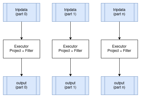
These operators are called “embarrassingly parallel” because parallelising them requires no special handling. The distributed plan looks just like the single-node plan, except different executors process different partitions. The partitioning scheme of the data does not change.

Distributed Aggregates

Aggregates require special handling in distributed execution. As discussed in the previous chapter, we split aggregation into two phases: a partial aggregate on each partition and a final aggregate that combines the partial results.

In distributed execution, the partial aggregates run on executors close to the data. The Exchange operator then moves partial results to where the final aggregation happens. For a query like:

SELECT passenger_count, MAX(fare_amount)
FROM tripdata
GROUP BY passenger_count

The distributed plan looks like:

HashAggregate: groupBy=[passenger_count], aggr=[MAX(fare_amount)]
  Exchange:
    HashAggregate: groupBy=[passenger_count], aggr=[MAX(fare_amount)]
      Scan: tripdata.parquet

Each executor runs the inner HashAggregate on its assigned partitions of tripdata. This produces partial results with far fewer rows than the input (one row per distinct passenger_count value per partition). The Exchange operator collects these partial results, and the outer HashAggregate combines them into the final answer.

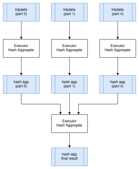
The exchange is the expensive part. Even though partial aggregation dramatically reduces data volume, we still need to transfer data over the network. For this query, we might reduce billions of input rows to thousands of partial aggregate rows, but those rows still need to reach whichever executor performs the final aggregation.

For aggregates grouped by high-cardinality columns (columns with many distinct values), the partial results may not be much smaller than the input. In extreme cases, the distributed overhead outweighs the benefit of distributing the initial scan.

Distributed Joins

Joins are often the most expensive operation in distributed query execution because they typically require shuffling large amounts of data across the network.

The challenge is that rows from both tables can only be joined if they are on the same executor. If we are joining customer to orders on customer.id = order.customer_id, then all orders for customer 12345 must be processed by the same executor that has customer 12345’s details.

Shuffle Join

When both tables are large, we use a shuffle join (also called a partitioned hash join). Both tables are repartitioned by the join key, ensuring that matching rows end up on the same executor.

The process has two stages:

Shuffle stage: Read both tables and redistribute rows based on a hash of the join key. All rows with the same join key value go to the same partition, and thus the same executor. This requires transferring potentially large amounts of data across the network.
Join stage: Each executor performs a local hash join on its partitions. Since all matching rows are now local, no further network communication is needed.

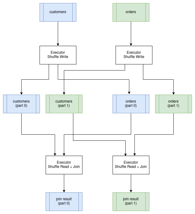
The shuffle is expensive. Every row from both tables must be sent over the network to its destination executor. For a join between two billion-row tables, this could mean transferring terabytes of data, even if the final result is small.

Broadcast Join

When one side of a join is small enough to fit in memory on each executor, we can avoid the shuffle entirely. The coordinator sends a copy of the small table to every executor. Each executor then joins its partitions of the large table against the local copy of the small table.

This trades network bandwidth (sending the small table everywhere) for avoiding the much larger cost of shuffling the big table. It only works when the small table is genuinely small, typically under a few gigabytes.

The query planner decides between shuffle and broadcast joins based on table size estimates. If statistics are available, it can make this decision automatically. Otherwise, users may need to provide hints.

Co-located Joins

If both tables are already partitioned by the join key (perhaps because they were written that way, or because a previous operation partitioned them), we can skip the shuffle entirely. Each executor joins its local partitions from both tables.

This is the fastest distributed join because no data moves. It requires careful data layout and is common in data warehouses where tables are deliberately partitioned by frequently-joined keys.

Query Stages

A distributed query cannot be executed as a single unit. The coordinator must break it into stages that can be executed independently, schedule those stages in the right order, and coordinate data flow between them.

A query stage is a portion of the query plan that can run to completion without waiting for other stages. Stages are separated by exchange operators, which represent points where data must be shuffled between executors. Within a stage, operators can be pipelined: data flows from one operator to the next without materialisation.

Consider the aggregate query from earlier:

HashAggregate: groupBy=[passenger_count], aggr=[MAX(fare_amount)]
  Exchange:
    HashAggregate: groupBy=[passenger_count], aggr=[MAX(fare_amount)]
      Scan: tripdata.parquet

This plan has two stages:

Stage 1: Scan the data and compute partial aggregates. This runs in parallel across all executors that have data partitions. Each executor reads its partitions, aggregates locally, and writes results to shuffle files.

Stage 2: Read the shuffle outputs from Stage 1 and compute the final aggregate. This might run on a single executor (for queries that need a single result) or on multiple executors (if the result is partitioned).

Stage 2 cannot start until Stage 1 completes because it reads Stage 1’s output. The coordinator tracks stage dependencies and schedules stages as their inputs become available.

Producing a Distributed Query Plan

Converting a logical plan into a distributed execution plan involves identifying where exchanges must occur and grouping operators into stages. The boundaries between stages occur where data must be repartitioned.

Consider this query joining customers with their orders:

SELECT customer.id, SUM(order.amount) AS total_amount
FROM customer JOIN order ON customer.id = order.customer_id
GROUP BY customer.id

The single-node physical plan looks like:

Projection: #customer.id, #total_amount
  HashAggregate: groupBy=[customer.id], aggr=[SUM(amount) AS total_amount]
    Join: condition=[customer.id = order.customer_id]
      Scan: customer
      Scan: order

To distribute this, we need to identify where exchanges occur. Assuming the tables are not already partitioned by customer id, the join requires shuffling both tables. The aggregate can run partially on each executor, but needs a final aggregation.

Stage 1 and 2 (run in parallel): Read and shuffle the input tables.

Stage #1: repartition=[customer.id]
  Scan: customer

Stage #2: repartition=[order.customer_id]
  Scan: order

Stage 3: Join the shuffled data and compute partial aggregates. Since the data is now partitioned by customer id, matching rows from both tables are on the same executor.

Stage #3: repartition=[]
  HashAggregate: groupBy=[customer.id], aggr=[SUM(amount) AS total_amount]
    Join: condition=[customer.id = order.customer_id]
      Stage #1 output
      Stage #2 output

Stage 4: Combine partial aggregates and project the final result.

Stage #4:
  Projection: #customer.id, #total_amount
    HashAggregate: groupBy=[customer.id], aggr=[SUM(total_amount)]
      Stage #3 output

The execution order is: Stages 1 and 2 run in parallel, then Stage 3, then Stage 4. Each stage boundary is an exchange where data is either shuffled (for the join) or gathered (for the final aggregation).

Serializing a Query Plan

The query scheduler needs to send fragments of the overall query plan to executors for execution.

There are a number of options for serializing a query plan so that it can be passed between processes. Many query engines choose the strategy of using the programming languages native serialization support, which is a suitable choice if there is no requirement to be able to exchange query plans between different programming languages and this is usually the simplest mechanism to implement.

However, there are advantages in using a serialization format that is programming language-agnostic. Ballista uses Google’s Protocol Buffers format to define query plans. The project is typically abbreviated as “protobuf”.

Here is a subset of the Ballista protocol buffer definition of a query plan.

Full source code can be found at proto/ballista.proto in the Ballista github repository.

message LogicalPlanNode {
  LogicalPlanNode input = 1;
  FileNode file = 10;
  ProjectionNode projection = 20;
  SelectionNode selection = 21;
  LimitNode limit = 22;
  AggregateNode aggregate = 23;
}

message FileNode {
  string filename = 1;
  Schema schema = 2;
  repeated string projection = 3;
}

message ProjectionNode {
  repeated LogicalExprNode expr = 1;
}

message SelectionNode {
  LogicalExprNode expr = 2;
}

message AggregateNode {
  repeated LogicalExprNode group_expr = 1;
  repeated LogicalExprNode aggr_expr = 2;
}

message LimitNode {
  uint32 limit = 1;
}

The protobuf project provides tools for generating language-specific source code for serializing and de-serializing data.

Serializing Data

Data must also be serialized as it is streamed between clients and executors and between executors.

Apache Arrow provides an IPC (Inter-process Communication) format for exchanging data between processes. Because of the standardized memory layout provided by Arrow, the raw bytes can be transferred directly between memory and an input/output device (disk, network, etc) without the overhead typically associated with serialization. This is effectively a zero copy operation because the data does not have to be transformed from its in-memory format to a separate serialization format.

However, the metadata about the data, such as the schema (column names and data types) does need to be encoded using Google Flatbuffers. This metadata is small and is typically serialized once per result set or per batch so the overhead is small.

Another advantage of using Arrow is that it provides very efficient exchange of data between different programming languages.

Apache Arrow IPC defines the data encoding format but not the mechanism for exchanging it. Arrow IPC could be used to transfer data from a JVM language to C or Rust via JNI for example.

Choosing a Protocol

Now that we have chosen serialization formats for query plans and data, the next question is how do we exchange this data between distributed processes.

Apache Arrow provides a Flight protocol which is intended for this exact purpose. Flight is a new general-purpose client-server framework to simplify high performance transport of large datasets over network interfaces.

The Arrow Flight libraries provide a development framework for implementing a service that can send and receive data streams. A Flight server supports several basic kinds of requests:

Handshake: a simple request to determine whether the client is authorized and, in some cases, to establish an implementation-defined session token to use for future requests
ListFlights: return a list of available data streams
GetSchema: return the schema for a data stream
GetFlightInfo: return an “access plan” for a dataset of interest, possibly requiring consuming multiple data streams. This request can accept custom serialized commands containing, for example, your specific application parameters.
DoGet: send a data stream to a client
DoPut: receive a data stream from a client
DoAction: perform an implementation-specific action and return any results, i.e. a generalized function call
ListActions: return a list of available action types

The GetFlightInfo method could be used to compile a query plan and return the necessary information for receiving the results, for example, followed by calls to DoGet on each executor to start receiving the results from the query.

Streaming vs Blocking Operators

Operators differ in whether they can stream results incrementally or must wait for all input before producing output.

Streaming operators produce output as soon as they receive input. Filter and projection are streaming: each input batch produces an output batch immediately. A pipeline of streaming operators can begin returning results while still reading input, reducing latency and memory usage.

Blocking operators must receive all input before producing any output. Sort is the clearest example: you cannot know which row comes first until you have seen all rows. Global aggregates (without GROUP BY) are similar: you cannot return the final SUM until all rows are processed.

Partially blocking operators fall in between. Hash join builds a hash table from one input (blocking on that side) but then streams through the other input. Hash aggregate accumulates results but can output partial aggregates incrementally when using two-phase aggregation.

In distributed execution, blocking operators create natural stage boundaries. All upstream work must complete before the blocking operator can produce its first output. This affects both latency (how long until results start appearing) and resource usage (intermediate data must be materialised).

Increasing the number of partitions helps reduce blocking time. Instead of one executor sorting a billion rows, we have a thousand executors each sorting a million rows. The merge step at the end is still necessary, but it operates on pre-sorted streams and can begin producing output immediately.

Data Locality

A key optimisation in distributed execution is moving computation to data rather than data to computation. Reading a terabyte over the network takes far longer than running a query locally on a terabyte of data.

When data lives in a distributed file system like HDFS, the coordinator knows which machines have local copies of each data block. It can assign tasks to executors that have the data locally, avoiding network transfer for the initial scan. This is called data locality or data affinity.

With cloud object stores like S3, data locality is less relevant because data must be fetched over the network regardless. However, executors in the same region as the storage will have lower latency and higher bandwidth than executors in different regions.

The shuffle operation between stages necessarily moves data across the network, so data locality only helps with the initial scan. For queries that are dominated by shuffles (complex joins, high-cardinality aggregates), locality provides less benefit.

Fault Tolerance

Long-running distributed queries face a significant risk: with hundreds of machines running for hours, the probability that at least one fails becomes high. Without fault tolerance, any failure means restarting the entire query from scratch.

There are several approaches to fault tolerance:

Checkpointing: Periodically save intermediate state to durable storage. If a failure occurs, restart from the most recent checkpoint rather than from the beginning. The trade-off is the overhead of writing checkpoints.

Lineage-based recovery: Instead of saving intermediate data, save the computation graph (lineage) that produced it. If data is lost, recompute it from its inputs. This is the approach used by Apache Spark. It works well when the lineage is not too long and recomputation is cheap.

Replication: Run multiple copies of each task on different machines. If one fails, use the results from another. This trades resource efficiency for reliability and is typically used for critical stages.

Task retry: If a task fails, simply re-run it (possibly on a different executor). This works for transient failures but requires the input data to still be available.

Most production systems combine these approaches. Early stages use lineage-based recovery (input data is durable on disk, so lost results can be recomputed). Expensive shuffle data may be replicated or checkpointed. Failed tasks are retried a few times before escalating to stage-level recovery.

Custom Code

It is often necessary to run user-defined functions as part of a distributed query. Serializing and shipping code to executors raises practical challenges.

For single-language systems, the language’s built-in serialization often works. Java can serialize lambda functions, Python can pickle functions (with caveats). The coordinator sends the serialized code along with the query plan.

For production systems, code is typically pre-deployed to executors. JVM systems might use Maven coordinates to download JARs. Container-based systems package dependencies into Docker images. The query plan then references the code by name rather than including it inline.

The user code must implement a known interface so the executor can invoke it. Type mismatches between the expected and actual interfaces cause runtime failures that can be hard to debug in a distributed setting.

Distributed Query Optimizations

The same query can be distributed in many ways. Choosing the best distribution requires estimating costs and making trade-offs.

Cost Factors

Distributed execution involves multiple scarce resources:

Network bandwidth: Shuffles transfer data between machines. Network is often the bottleneck, especially for join-heavy queries. Minimising shuffle size is usually the highest priority.

Memory: Each executor has limited memory. Hash tables for joins and aggregates must fit, or spill to disk at a severe performance cost. More executors means more aggregate memory, but also more coordination overhead.

CPU: Computation itself is parallelisable, but the benefit diminishes if the query is bottlenecked on I/O or network.

Disk I/O: Reading source data, writing shuffle files, and spilling all compete for disk bandwidth. SSDs help but have limits.

Monetary cost: In cloud environments, more executors means higher cost. A query that runs in 10 minutes on 100 executors might run in 15 minutes on 50 executors at half the price.

Optimisation Strategies

Shuffle minimisation: Choose join strategies that minimise data movement. Use broadcast joins when one side is small. Leverage co-located data when available. Filter early to reduce the data that reaches shuffles.

Predicate pushdown: Push filters as close to the data source as possible. If the storage system supports predicate pushdown (like Parquet with column statistics), even less data is read from disk.

Partition pruning: Skip partitions that cannot contain matching rows. Time-partitioned data benefits enormously when queries filter on time.

Statistics-based planning: With accurate statistics (row counts, column cardinalities, value distributions), the planner can estimate costs and choose better strategies. Without statistics, it must guess or use conservative defaults.

Adaptive Execution

An alternative to upfront cost estimation is adaptive execution: start running the query and adjust the plan based on observed data characteristics.

Apache Spark’s Adaptive Query Execution dynamically:

Coalesces small shuffle partitions to reduce overhead
Switches join strategies based on actual data sizes
Optimises skewed joins by splitting hot partitions

Adaptive execution is particularly valuable when statistics are unavailable or stale, which is common in data lake environments where new data arrives continuously.

The COST of Distribution

It bears repeating: distributed execution has overhead. The paper “Scalability! But at what COST?” (Configuration that Outperforms a Single Thread) demonstrates that many distributed systems are slower than a single well-optimised machine for medium-sized datasets.

Before scaling out to a cluster, ensure you have actually hit the limits of a single machine. Modern servers with hundreds of gigabytes of RAM and fast NVMe storage can process surprisingly large datasets. The complexity and operational overhead of distributed systems is only justified when the data truly exceeds single-machine capacity.

This book is also available for purchase in ePub, MOBI, and PDF format from https://leanpub.com/how-query-engines-work

Testing

The source code discussed in this chapter can be found in the test directories throughout the KQuery project.

Query engines are complex systems where subtle bugs can cause queries to return incorrect results. Unlike a crash or obvious error, a query that silently returns wrong data is particularly dangerous because users may make decisions based on faulty information. Rigorous testing is essential.

Why Query Engines Are Hard to Test

Several factors make testing query engines challenging:

The combinatorial explosion of operators and expressions means there are infinite ways to combine them. A simple query with three operators and two expressions per operator already has many possible combinations. Hand-written tests cannot cover them all.

Type coercion adds another dimension. An expression like a > b must work correctly for integers, floats, strings, dates, and more. Each comparison operator multiplied by each type combination multiplied by null handling creates many test cases.

Edge cases abound: empty tables, single-row tables, tables with all nulls, extremely large values, NaN for floating point, and Unicode strings with special characters. Production data will eventually exercise all of these.

Query optimizers can introduce bugs. A query might work correctly without optimization but fail after the optimizer rewrites it. Or the optimizer might produce a plan that is semantically different from the original.

Unit Testing

Unit tests verify that individual components work correctly in isolation. For a query engine, this means testing expressions, operators, and data sources independently before testing them in combination.

Testing Expressions

Expression tests should verify that each expression produces correct results for valid inputs and handles edge cases appropriately.

Here is a test for the greater-than-or-equals expression across different numeric types:

@Test
fun `gteq longs`() {
    val schema = Schema(listOf(
        Field("a", ArrowTypes.Int64Type),
        Field("b", ArrowTypes.Int64Type)
    ))

    val a: List<Long> = listOf(111, 222, 333, Long.MIN_VALUE, Long.MAX_VALUE)
    val b: List<Long> = listOf(111, 333, 222, Long.MAX_VALUE, Long.MIN_VALUE)

    val batch = Fuzzer().createRecordBatch(schema, listOf(a, b))

    val expr = GtEqExpression(ColumnExpression(0), ColumnExpression(1))
    val result = expr.evaluate(batch)

    assertEquals(a.size, result.size())
    (0 until result.size()).forEach {
        assertEquals(a[it] >= b[it], result.getValue(it))
    }
}

This test includes MIN_VALUE and MAX_VALUE to verify boundary behavior. Similar tests should exist for bytes, shorts, integers, floats, doubles, and strings. Each numeric type can have different overflow or comparison semantics.

For floating point types, testing NaN behavior is critical:

@Test
fun `gteq doubles`() {
    val schema = Schema(listOf(
        Field("a", ArrowTypes.DoubleType),
        Field("b", ArrowTypes.DoubleType)
    ))

    val a: List<Double> = listOf(0.0, 1.0,
        Double.MIN_VALUE, Double.MAX_VALUE, Double.NaN)
    val b = a.reversed()

    val batch = Fuzzer().createRecordBatch(schema, listOf(a, b))

    val expr = GtEqExpression(ColumnExpression(0), ColumnExpression(1))
    val result = expr.evaluate(batch)

    assertEquals(a.size, result.size())
    (0 until result.size()).forEach {
        assertEquals(a[it] >= b[it], result.getValue(it))
    }
}

NaN comparisons follow IEEE 754 semantics where NaN compared to anything (including itself) returns false. This surprises many developers, so explicit tests catch implementations that handle NaN incorrectly.

Creating Test Data

Tests need a convenient way to create record batches with arbitrary data. A helper method that takes a schema and column values makes tests cleaner:

fun createRecordBatch(schema: Schema, columns: List<List<Any?>>): RecordBatch {
    val rowCount = columns[0].size

    val root = VectorSchemaRoot.create(schema.toArrow(), rootAllocator)
    root.allocateNew()

    (0 until rowCount).forEach { row ->
        (0 until columns.size).forEach { col ->
            val v = root.getVector(col)
            val value = columns[col][row]
            when (v) {
                is BitVector -> v.set(row, if (value as Boolean) 1 else 0)
                is TinyIntVector -> v.set(row, value as Byte)
                is SmallIntVector -> v.set(row, value as Short)
                is IntVector -> v.set(row, value as Int)
                is BigIntVector -> v.set(row, value as Long)
                is Float4Vector -> v.set(row, value as Float)
                is Float8Vector -> v.set(row, value as Double)
                is VarCharVector -> v.set(row, (value as String).toByteArray())
                else -> throw IllegalStateException()
            }
        }
    }
    root.rowCount = rowCount

    return RecordBatch(schema, root.fieldVectors.map { ArrowFieldVector(it) })
}

With this helper, tests become declarative: define the schema, provide the data, and verify the result.

What to Test

Here are categories of unit tests that every query engine should have:

Type handling: What happens when an expression receives an unexpected type? For example, computing SUM on strings should produce a clear error.

Boundary values: Test minimum and maximum values for each numeric type. Test empty strings and very long strings.

Null handling: Every expression must handle null inputs correctly. Typically, any operation involving null produces null (SQL three-valued logic).

Overflow and underflow: What happens when multiplying two large integers overflows? The behavior should be documented and tested.

Special floating point values: Test positive and negative infinity, NaN, positive and negative zero.

Testing SQL Parsing

SQL parsing deserves dedicated tests because the parser is a critical component that interprets user queries. Parser bugs can cause queries to be misinterpreted, potentially with serious consequences.

Testing Operator Precedence

Mathematical expressions must respect operator precedence. These tests verify that multiplication binds tighter than addition:

@Test
fun `1 + 2 * 3`() {
    val expr = parse("1 + 2 * 3")
    val expected = SqlBinaryExpr(
        SqlLong(1),
        "+",
        SqlBinaryExpr(SqlLong(2), "*", SqlLong(3))
    )
    assertEquals(expected, expr)
}

@Test
fun `1 * 2 + 3`() {
    val expr = parse("1 * 2 + 3")
    val expected = SqlBinaryExpr(
        SqlBinaryExpr(SqlLong(1), "*", SqlLong(2)),
        "+",
        SqlLong(3)
    )
    assertEquals(expected, expr)
}

The tree structure of the parsed expression reveals which operations bind first. In 1 + 2 * 3, the 2 * 3 forms a subtree because multiplication has higher precedence.

Testing Query Structure

Tests should verify that each SQL clause is parsed correctly:

@Test
fun `parse SELECT with WHERE`() {
    val select = parseSelect(
        "SELECT id, first_name, last_name FROM employee WHERE state = 'CO'"
    )
    assertEquals(
        listOf(
            SqlIdentifier("id"),
            SqlIdentifier("first_name"),
            SqlIdentifier("last_name")
        ),
        select.projection
    )
    assertEquals(
        SqlBinaryExpr(SqlIdentifier("state"), "=", SqlString("CO")),
        select.selection
    )
    assertEquals("employee", select.tableName)
}

@Test
fun `parse SELECT with aggregates`() {
    val select = parseSelect(
        "SELECT state, MAX(salary) FROM employee GROUP BY state"
    )
    assertEquals(
        listOf(
            SqlIdentifier("state"),
            SqlFunction("MAX", listOf(SqlIdentifier("salary")))
        ),
        select.projection
    )
    assertEquals(listOf(SqlIdentifier("state")), select.groupBy)
}

Integration Testing

Integration tests verify that components work together correctly. For a query engine, this means executing complete queries and verifying the results.

End-to-End Query Tests

These tests exercise the full query path from parsing through execution:

@Test
fun `employees in CO using DataFrame`() {
    val ctx = ExecutionContext(mapOf())

    val df = ctx.csv(employeeCsv)
        .filter(col("state") eq lit("CO"))
        .project(listOf(col("id"), col("first_name"), col("last_name")))

    val batches = ctx.execute(df).asSequence().toList()
    assertEquals(1, batches.size)

    val batch = batches.first()
    assertEquals("2,Gregg,Langford\n" + "3,John,Travis\n", batch.toCSV())
}

@Test
fun `employees in CA using SQL`() {
    val ctx = ExecutionContext(mapOf())

    val employee = ctx.csv(employeeCsv)
    ctx.register("employee", employee)

    val df = ctx.sql(
        "SELECT id, first_name, last_name FROM employee WHERE state = 'CA'"
    )

    val batches = ctx.execute(df).asSequence().toList()
    assertEquals(1, batches.size)

    val batch = batches.first()
    assertEquals("1,Bill,Hopkins\n", batch.toCSV())
}

These tests use a small, static test file so the expected results are known. The CSV output format makes assertions readable and diff-friendly when tests fail.

Testing Complex Operations

Aggregation, joins, and other complex operations need thorough integration testing:

@Test
fun `aggregate query`() {
    val ctx = ExecutionContext(mapOf())

    val df = ctx.csv(employeeCsv)
        .aggregate(
            listOf(col("state")),
            listOf(Max(cast(col("salary"), ArrowType.Int(32, true))))
        )

    val batches = ctx.execute(df).asSequence().toList()
    assertEquals(1, batches.size)

    val batch = batches.first()
    val expected = "CO,11500\n" + "CA,12000\n" + ",11500\n"
    assertEquals(expected, batch.toCSV())
}

@Test
fun `inner join using DataFrame`() {
    val leftSchema = Schema(listOf(
        Field("id", ArrowTypes.Int32Type),
        Field("name", ArrowTypes.StringType)
    ))
    val rightSchema = Schema(listOf(
        Field("id", ArrowTypes.Int32Type),
        Field("dept", ArrowTypes.StringType)
    ))

    val leftData = Fuzzer().createRecordBatch(
        leftSchema,
        listOf(listOf(1, 2, 3), listOf("Alice", "Bob", "Carol"))
    )
    val rightData = Fuzzer().createRecordBatch(
        rightSchema,
        listOf(listOf(1, 2, 4), listOf("Engineering", "Sales", "Marketing"))
    )

    val leftSource = InMemoryDataSource(leftSchema, listOf(leftData))
    val rightSource = InMemoryDataSource(rightSchema, listOf(rightData))

    val ctx = ExecutionContext(mapOf())

    val leftDf = DataFrameImpl(Scan("left", leftSource, listOf()))
    val rightDf = DataFrameImpl(Scan("right", rightSource, listOf()))

    val joinedDf = leftDf.join(rightDf, JoinType.Inner, listOf("id" to "id"))

    val batches = ctx.execute(joinedDf).asSequence().toList()
    assertEquals(1, batches.size)

    val batch = batches.first()
    assertEquals(2, batch.rowCount())
    assertEquals("1,Alice,Engineering\n2,Bob,Sales\n", batch.toCSV())
}

The join test creates in-memory data sources to have precise control over the input data. This makes the expected output predictable and the test deterministic.

Comparative Testing

Comparative testing executes the same query against a trusted reference implementation and verifies that both produce the same results. This is particularly valuable for catching subtle bugs.

Common approaches include:

Running queries against PostgreSQL, DuckDB, or another established database and comparing results
Comparing DataFrame API queries against equivalent SQL queries within the same engine
Running optimized queries against unoptimized versions to verify the optimizer preserves semantics

The challenge with comparative testing is handling differences in null ordering, floating point precision, and result ordering when ORDER BY is not specified.

Fuzzing

Hand-written tests inevitably miss edge cases. Fuzzing generates random inputs to discover bugs that humans would not think to test.

Random Expression Generation

The fuzzer creates random expression trees by recursively building either leaf nodes (columns, literals) or binary expressions:

fun createExpression(input: DataFrame, depth: Int, maxDepth: Int): LogicalExpr {
    return if (depth == maxDepth) {
        // return a leaf node
        when (rand.nextInt(4)) {
            0 -> ColumnIndex(rand.nextInt(input.schema().fields.size))
            1 -> LiteralDouble(rand.nextDouble())
            2 -> LiteralLong(rand.nextLong())
            3 -> LiteralString(randomString(rand.nextInt(64)))
            else -> throw IllegalStateException()
        }
    } else {
        // binary expressions
        val l = createExpression(input, depth+1, maxDepth)
        val r = createExpression(input, depth+1, maxDepth)
        return when (rand.nextInt(8)) {
            0 -> Eq(l, r)
            1 -> Neq(l, r)
            2 -> Lt(l, r)
            3 -> LtEq(l, r)
            4 -> Gt(l, r)
            5 -> GtEq(l, r)
            6 -> And(l, r)
            7 -> Or(l, r)
            else -> throw IllegalStateException()
        }
    }
}

A depth limit prevents unbounded recursion. The random seed should be fixed for reproducibility.

Random Plan Generation

Similarly, the fuzzer can generate random query plans:

fun createPlan(input: DataFrame,
               depth: Int,
               maxDepth: Int,
               maxExprDepth: Int): DataFrame {

    return if (depth == maxDepth) {
        input
    } else {
        // recursively create an input plan
        val child = createPlan(input, depth+1, maxDepth, maxExprDepth)
        // apply a transformation to the plan
        when (rand.nextInt(2)) {
            0 -> {
                val exprCount = 1.rangeTo(rand.nextInt(1, 5))
                child.project(exprCount.map {
                    createExpression(child, 0, maxExprDepth)
                })
            }
            1 -> child.filter(createExpression(input, 0, maxExprDepth))
            else -> throw IllegalStateException()
        }
    }
}

Here is an example of a generated plan:

Filter: 'VejBmVBpYp7gHxHIUB6UcGx' OR 0.7762591612853446
  Filter: 'vHGbOKKqR' <= 0.41876514212913307
    Filter: 0.9835090312561898 <= 3342229749483308391
      Filter: -5182478750208008322 < -8012833501302297790
        Filter: 0.3985688976088563 AND #1
          Filter: #5 OR 'WkaZ54spnoI4MBtFpQaQgk'
            Scan: employee.csv; projection=None

Enhanced Random Values

Naive random number generation misses interesting edge cases. An enhanced random generator deliberately produces boundary values:

class EnhancedRandom(val rand: Random) {

    fun nextDouble(): Double {
        return when (rand.nextInt(8)) {
            0 -> Double.MIN_VALUE
            1 -> Double.MAX_VALUE
            2 -> Double.POSITIVE_INFINITY
            3 -> Double.NEGATIVE_INFINITY
            4 -> Double.NaN
            5 -> -0.0
            6 -> 0.0
            7 -> rand.nextDouble()
            else -> throw IllegalStateException()
        }
    }

    fun nextLong(): Long {
        return when (rand.nextInt(5)) {
            0 -> Long.MIN_VALUE
            1 -> Long.MAX_VALUE
            2 -> -0
            3 -> 0
            4 -> rand.nextLong()
            else -> throw IllegalStateException()
        }
    }
}

By weighting the distribution toward edge cases, the fuzzer finds bugs faster than pure random generation.

Handling Invalid Plans

Most randomly generated plans are invalid. This is actually useful because it tests error handling. However, if you want to test execution specifically, the fuzzer can be made “smarter” by:

Generating type-aware expressions (e.g., only compare compatible types)
Generating AND/OR expressions with Boolean operands
Ensuring aggregate expressions use aggregate functions

The trade-off is that smarter fuzzers may miss bugs in error paths.

Using Fuzzing Effectively

Some practical tips for fuzzing:

Fix the random seed: Use a constant seed so failures are reproducible. Log the seed if using system time.

Run many iterations: Fuzzing finds bugs probabilistically. Run thousands or millions of iterations.

Shrink failing cases: When fuzzing finds a bug, try to reduce the failing input to a minimal reproduction.

Keep regression tests: When fuzzing finds a bug, add the simplified case as a permanent test.

Golden Testing

Golden testing (also called snapshot testing) captures the output of a query and stores it as the expected result. Future runs compare against this “golden” output.

This approach works well for:

Query plan pretty-printing (verifying plan structure)
Explain output format
Error messages

The downside is that golden tests can be brittle. Any change to output formatting breaks the tests, even if the underlying behavior is correct.

Testing Optimizations

Optimizer bugs are particularly insidious because the unoptimized query works correctly. Test optimizations by:

Verifying that optimized and unoptimized plans produce identical results
Verifying that specific optimizations fire when expected
Testing that invalid optimizations do not fire

For example, to test projection push-down:

@Test
fun `projection pushdown reduces columns read`() {
    val plan = // build a plan that selects 3 columns from a 10 column table

    val optimized = Optimizer().optimize(plan)

    // Verify the scan only reads the 3 needed columns
    val scan = findScan(optimized)
    assertEquals(3, scan.projection.size)
}

@Test
fun `optimization preserves query semantics`() {
    val plan = // build a query plan
    val optimized = Optimizer().optimize(plan)

    val originalResult = execute(plan)
    val optimizedResult = execute(optimized)

    assertEquals(originalResult, optimizedResult)
}

Debugging Test Failures

When a test fails, the key is reproducing and understanding the failure.

Pretty-print plans: Implement a pretty() method on logical and physical plans. When a test fails, print the plan to understand what query was executed.

Log intermediate results: For debugging, add logging that shows data flowing through each operator.

Minimize the reproduction: Start with a failing query and systematically simplify it while keeping the failure. Remove unnecessary columns, filters, and joins until you have the smallest query that exhibits the bug.

Check boundary conditions: Many bugs occur at boundaries. If a test with 100 rows fails, try 0, 1, and 2 rows.

Verify test data: Sometimes the test itself is wrong. Double-check that the test data and expected results are correct.

Continuous Integration

Automated testing in CI catches regressions before they reach users. A good CI setup for a query engine includes:

Run all unit tests on every commit
Run integration tests on every pull request
Run longer fuzzing sessions nightly or weekly
Track test execution time to catch performance regressions

Test failures should block merging. Flaky tests (tests that sometimes pass and sometimes fail) must be fixed immediately because they train developers to ignore failures.

Summary

Testing query engines requires multiple complementary approaches. Unit tests verify individual components. Integration tests verify components work together. Fuzzing discovers edge cases that humans miss. Comparative testing catches semantic bugs by checking against a reference implementation.

Invest in testing infrastructure early. Good test utilities (for creating test data, comparing results, pretty-printing plans) make writing tests easier, which means more tests get written. A well-tested query engine gives users confidence that their query results are correct.

This book is also available for purchase in ePub, MOBI, and PDF format from https://leanpub.com/how-query-engines-work

Benchmarks

Each query engine is unique in terms of performance, scalability, and resource requirements, often with different trade-offs. Benchmarks help us understand these characteristics and make informed decisions about which query engine to use for a particular workload. They also help query engine developers identify performance regressions and track improvements over time.

Measuring Performance

Performance is often the simplest characteristic to measure and usually refers to the time it takes to perform a particular operation. For example, benchmarks can be built to measure the performance of specific queries or categories of query.

Performance tests typically involve executing a query multiple times and measuring elapsed time.

Measuring Scalability

Scalability can be an overloaded term and there are many different types of scalability. The term scalability generally refers to how performance varies with different values for some variable that affects performance.

One example would be measuring scalability as total data size increases to discover how performance is impacted, when querying 10 GB of data versus 100 GB or 1 TB. A common goal is to demonstrate linear scalability, meaning that querying 100 GB of data should take 10 times as long as querying 10 GB of data. Linear scalability makes it easy for users to reason about expected behavior.

Other examples of variables that affect performance are:

Number of concurrent users, requests, or queries.
Number of data partitions.
Number of physical disks.
Number of cores.
Number of nodes.
Amount of RAM available.
Type of hardware (Raspberry Pi versus Desktop, for example).

Concurrency

When measuring scalability based on number of concurrent requests, we are often more interested in throughput (total number of queries executed per period of time) rather than the duration of individual queries, although we typically would collect that information as well.

Automation

Benchmarks are often very time-consuming to run and automation is essential so that the benchmarks can be run often, perhaps once per day or once per week, so that any performance regressions can be caught early.

Automation is also important for ensuring that benchmarks are executed consistently and that results are collected with all relevant details that might be needed when analyzing the results.

Here are some examples of the type of data that should be collected when executing benchmarks:

Hardware Configuration

Type of hardware
Number of CPU cores
Available memory and disk space
Operating system name and version

Environment

Environment variables (being careful not to leak secrets)

Benchmark Configuration

Version of benchmark software used
Version of software under test
Any configuration parameters or files
Filenames of any data files being queried
Data sizes and checksums for the data files
Details about the query that was executed

Benchmark Results

Date/time benchmark was started
Start time and end time for each query
Error information for any failed queries

Comparing Benchmarks

It is important to compare benchmarks between releases of the software so that changes in performance characteristics are apparent and can be investigated further. Benchmarks produce a lot of data that is often hard to compare manually, so it can be beneficial to build tooling to help with this process.

Rather than comparing two sets of performance data directly, tooling can perform a “diff” of the data and show percentage differences between two or more runs of the same benchmark. It is also useful to be able to produce charts showing multiple benchmark runs.

Visualising Benchmark Results

Raw benchmark data in tabular form can be difficult to interpret. Charts and graphs make it much easier to see patterns, identify anomalies, and communicate results to others.

When visualising performance data, consider charting throughput rather than raw execution times. Throughput, often expressed as queries per minute or queries per second, provides a more intuitive measure of system capacity. If a query takes 5 seconds to execute, then the system can handle 12 queries per minute on a single thread. This framing makes it easier to understand real-world capacity.

Line charts work well for showing how performance scales with increasing resources such as CPU cores or memory, or with increasing data sizes. Bar charts are useful for comparing different configurations or different query engines side by side.

Be careful when creating visualisations to use appropriate scales. Starting a y-axis at zero rather than at some arbitrary value gives a more honest representation of differences between data points. Using logarithmic scales can be appropriate when dealing with data that spans several orders of magnitude.

Transaction Processing Council (TPC) Benchmarks

The Transaction Processing Council is a consortium of database vendors that collaborate on creating and maintaining various database benchmark suites to allow for fair comparisons between vendor’s systems. Current TPC member companies include Microsoft, Oracle, IBM, Hewlett Packard Enterprise, AMD, Intel, and NVIDIA.

The first benchmark, TPC-A, was published in 1989 and other benchmarks have been created since then. TPC-C is a well known OLTP benchmark used when comparing traditional RDBMS databases, and TPC-H (discontinued) and TPC-DS are often used for measuring performance of “Big Data” query engines.

TPC benchmarks are seen as the “gold standard” in the industry and are complex and time consuming to implement fully. Also, results for these benchmarks can only be published by TPC members and only after the benchmarks have been audited by the TPC. Taking TPC-DS as an example, the only companies to have ever published official results at the time of writing are Alibaba.com, H2C, SuperMicro, and Databricks.

However, the TPC has a Fair Use policy that allows non-members to create unofficial benchmarks based on TPC benchmarks, as long as certain conditions are followed, such as prefixing any use of the term TPC with “derived from TPC”. For example, “Performance of Query derived from TPC-DS Query 14”. TPC Copyright Notice and License Agreements must also be maintained. There are also limitations on the types of metrics that can be published.

Many open source projects simply measure the time to execute individual queries from the TPC benchmark suites and use this as a way to track performance over time and for comparison with other query engines.

Common Pitfalls

There are several common mistakes to avoid when designing and running benchmarks.

The first run of a query is often slower than subsequent runs due to JIT compilation, cache population, and other startup effects. Running several warm-up iterations before collecting measurements helps ensure that results reflect steady-state performance rather than cold-start behaviour.

Running benchmarks on a machine that is also doing other work can introduce significant variability. Dedicated benchmark environments, or at least ensuring minimal background activity, produce more reliable results.

Running a query once and reporting that single result tells you very little. Running multiple iterations and reporting statistics such as mean, median, and standard deviation gives a much better picture of typical performance and its variability.

Benchmarks that use tiny datasets or trivially simple queries may not reveal performance characteristics that matter for real workloads. Using realistic data sizes and query complexity is important for meaningful results.

It can be tempting to only show results that make your query engine look good, but publishing complete results, including queries where performance is poor, builds credibility and helps identify areas for improvement.

Building Your Own Benchmarks

While industry-standard benchmarks like TPC-DS are valuable for comparing different systems, they may not reflect your specific workload. Building custom benchmarks based on real queries from your application can provide more relevant insights.

When building custom benchmarks, start by identifying the queries that matter most to your users. These might be the most frequently executed queries, or the queries that are most sensitive to latency. Instrument your application to collect query logs, then select representative queries for benchmarking.

Create datasets that match your production data in terms of size, distribution, and schema complexity. Synthetic data generators can help create large datasets with controlled characteristics, but be aware that randomly generated data may have different statistical properties than real data.

Document your benchmark methodology thoroughly so that results can be reproduced. This includes not just the queries and data, but also the hardware, operating system, and any configuration settings that might affect performance.

This book is also available for purchase in ePub, MOBI, and PDF format from https://leanpub.com/how-query-engines-work

Further Resources

I hope that you found this book useful and that you now have a better understanding of the internals of query engines. If there are topics that you feel haven’t been covered adequately, or at all, I would love to hear about it so I can consider adding additional content in a future revision of this book.

Feedback can be posted on the public forum on the Leanpub site, or you can message me directly via twitter at @andygrove_io.

Open-Source Projects

There are numerous open-source projects that contain query engines and working with these projects is a great way to learn more about the topic. Here are just a few examples of popular open-source query engines.

Apache Arrow
Apache Calcite
Apache Drill
Apache Hadoop
Apache Hive
Apache Impala
Apache Spark
Facebook Presto
NVIDIA RAPIDS Accelerator for Apache Spark

YouTube

I only recently discovered Andy Pavlo’s lecture series, which is available on YouTube (here). This covers much more than just query engines, but there is extensive content on query optimization and execution. I highly recommend watching these videos.

Sample Data

Earlier chapters reference the New York City Taxi & Limousine Commission Trip Record Data data set. The yellow and green taxi trip records include fields capturing pick-up and drop-off dates/times, pick-up and drop-off locations, trip distances, itemized fares, rate types, payment types, and driver-reported passenger counts.

When this book was first published, the data was provided in CSV format, but has now been converted to Parquet format. It is still possible to find the CSV versions of these files online. As of December 2025, the following locations contain this data:

https://github.com/DataTalksClub/nyc-tlc-data/releases
https://catalog.data.gov/dataset/2019-yellow-taxi-trip-data
https://www.kaggle.com/code/haydenbailey/newyork-yellow-taxi

The KQuery project contains source code for converting these CSV files into Parquet format. This book is also available for purchase in ePub, MOBI, and PDF format from https://leanpub.com/how-query-engines-work

Keyboard shortcuts

How Query Engines Work