Distributed Query Execution
The previous section on Parallel Query Execution covered some fundamental concepts such as partitioning, which we will build on in this section.
To somewhat over-simplify the concept of distributed query execution, the goal is to be able to create a physical query plan which defines how work is distributed to a number of “executors” in a cluster. Distributed query plans will typically contain new operators that describe how data is exchanged between executors at various points during query execution.
In the following sections we will explore how different types of plans are executed in a distributed environment and then discuss building a distributed query scheduler.
Embarrassingly Parallel Operators
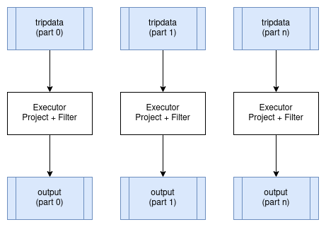
Certain operators can run in parallel on partitions of data without any significant overhead when running in a distributed environment. The best examples of these are Projection and Filter. These operators can be applied in parallel to each input partition of the data being operated on and produce a corresponding output partition for each one. These operators do not change the partitioning scheme of the data.
Distributed Aggregates
Let’s use the example SQL query that we used in the previous chapter on Parallel Query Execution and look at the distributed planning implications of an aggregate query.
SELECT passenger_count, MAX(max_fare)
FROM tripdata
GROUP BY passenger_count
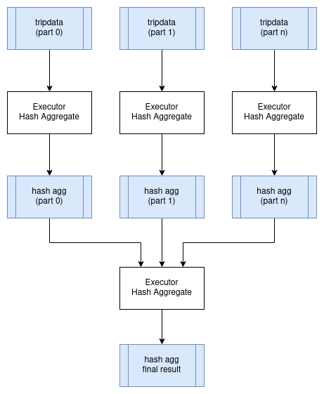
We can execute this query in parallel on all partitions of the tripdata table, with each executor in the cluster processing a subset of these partitions. However, we need to then combine all the resulting aggregated data onto a single node and then apply the final aggregate query so that we get a single result set without duplicate grouping keys (passenger_count in this case). Here is one possible logical query plan for representing this. Note the new Exchange operator which represents the exchange of data between executors. The physical plan for the exchange could be implemented by writing intermediate results to shared storage, or perhaps by streaming data directly to other executors.
HashAggregate: groupBy=[passenger_count], aggr=[MAX(max_fare)]
  Exchange:
    HashAggregate: groupBy=[passenger_count], aggr=[MAX(max_fare)]
      Scan: tripdata.parquet
Here is a diagram showing how this query could be executed in a distributed environment:
Distributed Joins
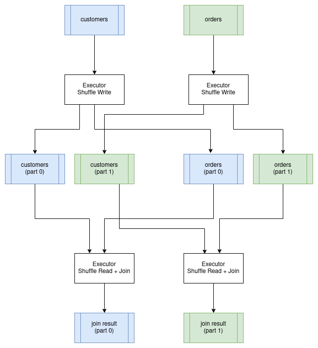
Joins are often the most expensive operation to perform in a distributed environment. The reason for this is that we need to make sure that we organize the data in such a way that both input relations are partitioned on the join keys. For example, if we joining a customer table to an order table where the join condition is customer.id = order.customer_id, then all the rows in both tables for a specific customer must be processed by the same executor. To achieve this, we have to first repartition both tables on the join keys and write the partitions to disk. Once this has completed then we can perform the join in parallel with one join for each partition. The resulting data will remain partitioned by the join keys. This particular join algorithm is called a partitioned hash join. The process of repartitioning the data is known as performing a “shuffle”.
Distributed Query Scheduling
Distributed query plans are fundamentally different to in-process query plans because we can’t just build a tree of operators and start executing them. The query now requires co-ordination across executors which means that we now need to build a scheduler.
At a high level, the concept of a distributed query scheduler is not complex. The scheduler needs to examine the whole query and break it down into stages that can be executed in isolation (usually in parallel across the executors) and then schedule these stages for execution based on the available resources in the cluster. Once each query stage completes then any subsequent dependent query stages can be scheduled. This process repeats until all query stages have been executed.
The scheduler could also be responsible for managing the compute resources in the cluster so that extra executors can be started on demand to handle the query load.
In the remainder of this chapter, we will discuss the following topics, referring to Ballista and the design that is being implemented in that project.
- Producing a distributed query plan
- Serializing query plans and exchanging them with executors
- Exchange intermediate results between executors
- Optimizing distributed queries
Producing a Distributed Query Plan
As we have seen in the previous examples, some operators can run in parallel on input partitions and some operators require data to be repartitioned. These changes in partitioning are key to planning a distributed query. Changes in partitioning within a plan are sometimes called pipeline breakers and these changes in partitioning define the boundaries between query stages.
We will now use the following SQL query to see how this process works.
SELECT customer.id, sum(order.amount) as total_amount
FROM customer JOIN order ON customer.id = order.customer_id
GROUP BY customer.id
The physical (non-distributed) plan for this query would look something like this:
Projection: #customer.id, #total_amount
  HashAggregate: groupBy=[customer.id], aggr=[MAX(max_fare) AS total_amount]
    Join: condition=[customer.id = order.customer_id]
      Scan: customer
      Scan: order
Assuming that the customer and order tables are not already partitioned on customer id, we will need to schedule execution of the first two query stages to repartition this data. These two query stages can run in parallel.
Query Stage #1: repartition=[customer.id]
  Scan: customer
Query Stage #2: repartition=[order.customer_id]
  Scan: order
Next, we can schedule the join, which will run in parallel for each partition of the two inputs. The next operator after the join is the aggregate, which is split into two parts; the aggregate that runs in parallel and then the final aggregate that requires a single input partition. We can perform the parallel part of this aggregate in the same query stage as the join because this first aggregate does not care how the data is partitioned. This gives us our third query stage, which can now be scheduled for execution. The output of this query stage remains partitioned by customer id.
Query Stage #3: repartition=[]
  HashAggregate: groupBy=[customer.id], aggr=[MAX(max_fare) AS total_amount]
    Join: condition=[customer.id = order.customer_id]
      Query Stage #1
      Query Stage #2
The final query stage performs the aggregate of the aggregates, reading from all of the partitions from the previous stage.
Query Stage #4:
  Projection: #customer.id, #total_amount
    HashAggregate: groupBy=[customer.id], aggr=[MAX(max_fare) AS total_amount]
      QueryStage #3
To recap, here is the full distributed query plan showing the query stages that are introduced when data needs to be repartitioned or exchanged between pipelined operations.
Query Stage #4:
  Projection: #customer.id, #total_amount
    HashAggregate: groupBy=[customer.id], aggr=[MAX(max_fare) AS total_amount]
      Query Stage #3: repartition=[]
        HashAggregate: groupBy=[customer.id], aggr=[MAX(max_fare) AS total_amount]
          Join: condition=[customer.id = order.customer_id]
            Query Stage #1: repartition=[customer.id]
              Scan: customer
            Query Stage #2: repartition=[order.customer_id]
              Scan: order
Serializing a Query Plan
The query scheduler needs to send fragments of the overall query plan to executors for execution.
There are a number of options for serializing a query plan so that it can be passed between processes. Many query engines choose the strategy of using the programming languages native serialization support, which is a suitable choice if there is no requirement to be able to exchange query plans between different programming languages and this is usually the simplest mechanism to implement.
However, there are advantages in using a serialization format that is programming language-agnostic. Ballista uses Google’s Protocol Buffers format to define query plans. The project is typically abbreviated as “protobuf”.
Here is a subset of the Ballista protocol buffer definition of a query plan.
Full source code can be found at proto/ballista.proto in the Ballista github repository.
message LogicalPlanNode {
  LogicalPlanNode input = 1;
  FileNode file = 10;
  ProjectionNode projection = 20;
  SelectionNode selection = 21;
  LimitNode limit = 22;
  AggregateNode aggregate = 23;
}

message FileNode {
  string filename = 1;
  Schema schema = 2;
  repeated string projection = 3;
}

message ProjectionNode {
  repeated LogicalExprNode expr = 1;
}

message SelectionNode {
  LogicalExprNode expr = 2;
}

message AggregateNode {
  repeated LogicalExprNode group_expr = 1;
  repeated LogicalExprNode aggr_expr = 2;
}

message LimitNode {
  uint32 limit = 1;
}
The protobuf project provides tools for generating language-specific source code for serializing and de-serializing data.
Serializing Data
Data must also be serialized as it is streamed between clients and executors and between executors.
Apache Arrow provides an IPC (Inter-process Communication) format for exchanging data between processes. Because of the standardized memory layout provided by Arrow, the raw bytes can be transferred directly between memory and an input/output device (disk, network, etc) without the overhead typically associated with serialization. This is effectively a zero copy operation because the data does not have to be transformed from its in-memory format to a separate serialization format.
However, the metadata about the data, such as the schema (column names and data types) does need to be encoded using Google Flatbuffers. This metadata is small and is typically serialized once per result set or per batch so the overhead is small.
Another advantage of using Arrow is that it provides very efficient exchange of data between different programming languages.
Apache Arrow IPC defines the data encoding format but not the mechanism for exchanging it. Arrow IPC could be used to transfer data from a JVM language to C or Rust via JNI for example.
Choosing a Protocol
Now that we have chosen serialization formats for query plans and data, the next question is how do we exchange this data between distributed processes.
Apache Arrow provides a Flight protocol which is intended for this exact purpose. Flight is a new general-purpose client-server framework to simplify high performance transport of large datasets over network interfaces.
The Arrow Flight libraries provide a development framework for implementing a service that can send and receive data streams. A Flight server supports several basic kinds of requests:
- Handshake: a simple request to determine whether the client is authorized and, in some cases, to establish an implementation-defined session token to use for future requests
- ListFlights: return a list of available data streams
- GetSchema: return the schema for a data stream
- GetFlightInfo: return an “access plan” for a dataset of interest, possibly requiring consuming multiple data streams. This request can accept custom serialized commands containing, for example, your specific application parameters.
- DoGet: send a data stream to a client
- DoPut: receive a data stream from a client
- DoAction: perform an implementation-specific action and return any results, i.e. a generalized function call
- ListActions: return a list of available action types
The GetFlightInfo method could be used to compile a query plan and return the necessary information for receiving the results, for example, followed by calls to DoGet on each executor to start receiving the results from the query.
Streaming
It is important that results of a query can be made available as soon as possible and be streamed to the next process that needs to operate on that data, otherwise there would be unacceptable latency involved as each operation would have to wait for the previous operation to complete.
However, some operations require all the input data to be received before any output can be produced. A sort operation is a good example of this. It isn’t possible to completely sort a dataset until the whole data set has been received. The problem can be alleviated by increasing the number of partitions so that a large number of partitions are sorted in parallel and then the sorted batches can be combined efficiently using a merge operator.
Custom Code
It is often necessary to run custom code as part of a distributed query or computation. For a single language query engine it is often possible to use the language’s built-in serialization mechanism to transmit this code over the network at query execution time which is very convenient during development. Another approach is to publish compiled code to a repository so that it can be downloaded into a cluster at runtime. For JVM based systems, a maven repository could be used. A more general purpose approach is to package all runtime dependencies into a Docker image.
The query plan needs to provide the necessary information to load the user code at runtime. For JVM based systems this could be a classpath and a class name. For C based systems, this could be the path to a shared object. In either case, the user code will need to implement some known API.
Distributed Query Optimizations
Distributed query execution has a lot of overhead compared to parallel query execution on a single host and should only be used when there is benefit in doing so. I recommend reading the paper Scalability! But at what COST for some interesting perspectives on this topic.
Also, there are many ways to distribute the same query so how do we know which one to use?
One answer is to build a mechanism to determine the cost of executing a particular query plan and then create some subset of all possible combinations of query plan for a given problem and determine which one is most efficient.
There are many factors involved in computing the cost of an operation and there are different resource costs and limitations involved.
- Memory: We are typically concerned with availability of memory rather than performance. Processing data in memory is orders of magnitude faster than reading and writing to disk.
- CPU: For workloads that are parallelizable, more CPU cores means better throughput.
- GPU: Some operations are orders of magnitude faster on GPUs compared to CPUs.
- Disk: Disks have finite read and write speeds and cloud vendors typically limit the number of I/O operations per second (IOPS). Different types of disk have different performance characteristics (spinning disk vs SSD vs NVMe).
- Network: Distributed query execution involves streaming data between nodes. There is a throughput limitation imposed by the networking infrastructure.
- Distributed Storage: It is very common for source data to be stored in a distributed file system (HDFS) or object store (Amazon S3, Azure Blob Storage) and there is a cost in transferring data between distributed storage and local file systems.
- Data Size: The size of the data matters. When performing a join between two tables and data needs to be transferred over the network, it is better to transfer the smaller of the two tables. If one of the tables can fit in memory than a more efficient join operation can be used.
- Monetary Cost: If a query can be computed 10% faster at 3x the cost, is it worth it? That is a question best answered by the user of course. Monetary costs are typically controlled by limiting the amount of compute resource that is available.
Query costs can be computed upfront using an algorithm if enough information is known ahead of time about the data, such as how large the data is, the cardinality of the partition of join keys used in the query, the number of partitions, and so on. This all depends on certain statistics being available for the data set being queried.
Another approach is to just start running a query and have each operator adapt based on the input data it receives. Apache Spark 3.0.0 introduced an Adaptive Query Execution feature that does just this.
This book is also available for purchase in ePub, MOBI, and PDF format from https://leanpub.com/how-query-engines-work
Copyright © 2020-2025 Andy Grove. All rights reserved.